---

---

Today, I’ll try to explain factorial experiments in the simplest way. When you apply multiple different factors simultaneously to derive experimental results, it’s called factorial experiments. The different treatments within the experiment are referred to as ‘factorials.’ In other words, a factorial is a combination of factors.

[Note 1]
A factorial experiment is a research design in which multiple independent variables, also known as factors, are manipulated simultaneously to analyze their combined effects on a dependent variable. The goal of a factorial experiment is to understand how different factors interact with one another and how they collectively influence the outcome or response being studied. 

Let’s take an example. Imagine we have two different cultivars (Cultivar 1, Cultivar 2) and four different nitrogen fertilizers (N0, N1, N2, N3). We want to see how the yield varies based on these combinations. The experiments were repeated in blocks, with three blocks in total.

---

[Note 2] Basic statistical terms

1) What are the experimental factors, and how many levels are there in each factor?
Factor 1 = Cultivar (2 level; Cultivar 1, Cultivar 2)
Factor 2 = Nitrogen (4 level; N0, N1, N2, N3)

2) How many treatments in total?
Treatment = 2 level x 4 level = 8 treatments (Number of experimental combinations)

3) How many experimental units in total?
Experimental unit = 2 level x 4 level x 3 block = 24 experimental units (Number of observations)

4) Which experimental design should be used?
Since repetitions are assigned to blocks, the experimental design should be planned using the Randomized Complete Block Design (RCBD).

5) Which statistical analysis method should be used?
Since it's an experiment to investigate whether two different factors affect the yield, a Two-way ANOVA (Two-way Analysis of Variance) should be conducted.

---

And I obtained the following results from the investigation of the yield:

   Cultivar Nitrogen Block Yield
1       CV1       N0     I    99
2       CV1       N0    II   109
3       CV1       N0   III    89
4       CV1       N1     I   115
5       CV1       N1    II   142
6       CV1       N1   III   133
7       CV1       N2     I   121
8       CV1       N2    II   157
9       CV1       N2   III   142
10      CV1       N3     I   125
11      CV1       N3    II   150
12      CV1       N3   III   139
13      CV2       N0     I    82
14      CV2       N0    II   104
15      CV2       N0   III    99
16      CV2       N1     I   117
17      CV2       N1    II   125
18      CV2       N1   III   127
19      CV2       N2     I   145
20      CV2       N2    II   154
21      CV2       N2   III   154
22      CV2       N3     I   151
23      CV2       N3    II   166
24      CV2       N3   III   175


# Download the above data to Excel using R.
Cultivar= rep(c("CV1","CV2"),each=12)
Nitrogen= rep(rep(c("N0","N1","N2","N3"), each=3),2)
Block= rep(c("I","II","III"),8)
Yield= c (99, 109, 89, 115, 142, 133, 121, 157, 142, 125, 150, 139, 82, 104, 99, 117, 125, 127, 145, 154, 154, 151, 166, 175)
dataA= data.frame(Cultivar,Nitrogen,Block,Yield)

library(writexl)
write_xlsx (dataA,"C:/Users/Usuari/Desktop/dataA.xlsx")
# Please confirm the directory path on your computer

---

---

With this data, I want to investigate whether the cultivar and nitrogen fertilizer bring about differences in yield. As always mentioned, using statistical software yields results in just a matter of seconds. However, what’s important is understanding the principles. Step by step, we’ll explore how statistical software derives results. Let’s start by understanding the mathematical model for this data structure.

yijk = μ + τij + γk + εijk

Where:
yijk represents the observed value for a specific combination of factors i(=cultivar), j(=nitrogen), and k(=replicates).
μ is the overall mean or baseline value.
τij represents the effect of the i-th cultivar and j-th nitrogen fertilizer.
γk represents the effect of the k-th block or repetition.
εijk is the error term, accounting for random variability and uncontrolled factors.

And the structure of the treatment τ_ij is further subdivided as shown below.

τij = αi + βj + δij

In other words, our data consisted of yield results for cultivar and nitrogen, and the experiment was conducted using RCBD (Randomized Complete Block Design). Therefore, the treatment outcomes relate to the differences in yield for each cultivar (α) and nitrogen (β), as well as the yield differences due to the interaction between cultivar and nitrogen (δ).

---

In that case, we can rephrase it using the following equation:

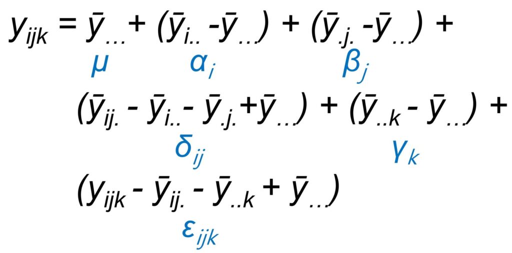
yijk = μ  + αi + βj + δij + γk + εijk

Where:    
yijk represents the observed value for a specific combination of factors i(=cultivar), j(=nitrogen), and k(=replicates).
μ is the overall mean or baseline value.
αi represents the effect of the i-th level of the cultivar (Cultivar i) on the observed variable. It captures how different cultivars influence the response variable.
βj represents the effect of the j-th level of the nitrogen fertilizer (Nitrogen j) on the observed variable. It indicates how different levels of nitrogen affect the response variable.
δij represents the interaction effect between the i-th level of cultivar and the j-th level of nitrogen. It shows whether the combined effect of cultivar and nitrogen is different from what would be expected from the individual effects.
γk represents the effect of the k-th block or repetition. In a randomized complete block design (RCBD), blocks are used to control potential sources of variation that are not of interest. This term accounts for any variation introduced by the different blocks.
εijk is the error term, representing the random variability and uncontrolled factors that affect the observed value. It encompasses any sources of variation that are not accounted for by the other terms in the equation.

Even though this equation might look complex, in reality, it’s as simple as basic addition and subtraction. You can actually rewrite it into the following calculation:

---

---

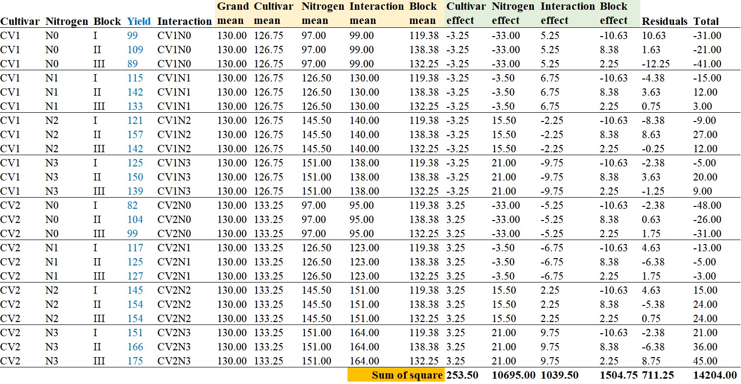
Let’s break down this calculation using Excel step by step.

I have uploaded the data as a .csv file on my GitHub. For those who need it, feel free to download and practice.

Download
https://github.com/agronomy4future/raw_data_practice/blob/main/example_residual_calculation.csv

(1) Grand mean (ȳ_…)
This is the average of the total yield values. Here, it’s 130.0.

(2) Cultivar mean (ȳ_i..)
These are the average yield values for each cultivar. Here, for CV1, it’s 126.75, and for CV2, it’s 133.25.

(3) Nitrogen mean (ȳ_.j.)
These are the average yield values for each nitrogen level. Here, for N0, it’s 97.0, for N1, it’s 126.5, for N2, it’s 145.5, and finally, for N3, it’s 151.0.

(4) Interaction mean (ȳ_ij.)
These are the average yield values when cultivar and nitrogen treatments are combined. For example, for CV1*N0, the average yield value is 99.0.

(5) Block mean (ȳ_..k)
The averages are as follows: for Block 1, it’s 119.4; for Block 2, it’s 138.4; and for Block 3, it’s 132.3.

(6) Cultivar effect (ȳ_i..– ȳ_…) = α_i
The concept of the “Cultivar effect” essentially involves comparing the average of each cultivar with the overall mean. The average for CV1 was 126.75, and for Cultivar 2, it was 133.25. Therefore, the effect of CV1 would be 126.75 – 130.0, resulting in -3.25. The effect of Cultivar 2 would be 133.25 – 130.0, resulting in 3.25.

(7) Nitrogen effect (ȳ_.j.– ȳ_…) = β_j
Using the same concept, we examine the difference between the average of N0 to N3 and the overall mean.

(8) Interaction effect Interaction (ȳ_ij. – ȳ_i.. – ȳ_.j. + ȳ_…) = δ_ij
For each interaction (CV1N0, … CV2N3), we examine the difference between the average of the interaction and the overall mean. To do this, we subtract the average of Cultivar 1 and the average of N0 from the average of the interaction, and then add the overall mean. For instance, considering CV1N0: the interaction effect for CV1N0 is calculated as 99.0 (average of CV1*N0) – 126.75 (average of Cultivar 1) – 97.0 (average of N0) + 130.0 (overall mean) = 5.25.

(9) Block effect (ȳ_..k – ȳ_…) = γ_k
We examine the difference between the average of each block and the overall mean.

(10) Residual (ȳ_ijk – ȳ_ij.– ȳ_..k + ȳ_…) = ε_ijk
The value for error is calculated for each yield value by subtracting the corresponding interaction and block averages, and then adding the overall mean. For instance, consider the yield value of 99 for CV1 and N1 in the first block: the error is calculated as 99 (yield value) – 99 (average of CV1*N1 interaction) – 119.4 (average of Block 1) + 130 (overall mean) = 10.63.

(11) Total (ȳ_ijk – ȳ_…)
While labeled as “Total,” a more accurate representation would be the variation of the entire dataset. In essence, it shows how much each yield value deviates from the mean. In other words, it involves subtracting the overall mean from each yield value.

---

---

Each yield value is partitioned using the equation mentioned above. For instance, the yield value of 99 for CV1 and N1 in the first block can be partitioned as follows:

99 = 130 + (126.75 – 130) + (97.0 – 130) + (99 – 126.75 – 97 + 130) + (119.4 – 130) + (99 – 99 – 119.4 + 130)

This partitioning represents how the total variation in each yield value can be attributed to different factors and interactions, as described by the equation.

That is, y111 = μ  + αi + βj + δij + γk + εijk

99 = 130 + (-3.25) + (-33.0) + 5.25 + (-10.6) + 10.63 is the breakdown.

Now, let’s calculate the sum of squares (SS) for these partitioned values. You might be wondering why we need to calculate the sum of squares (SS), but in fact, this is one of the most fundamental concepts in statistics.

---

[Note 2] Variance 
Let's say we have the observation values 4, 7, 6, and 3. The mean of these values is 5. We want to understand how far our data is from the mean. So, we subtracted the mean from each individual observation value. These differences are called deviations.

4 - 5 = -1
7 - 5 = 2
6 - 5 = 1
3 - 5 = -2

When we sum these deviations, we get 0. The sum of deviations is always 0. To prevent the sum of deviations from being 0, we square each deviation and then sum those squared values.

(-1)² + (2)² + (1)² + (-2)² = 10

By squaring and summing, we estimate how much our data deviates from the mean. This is why it's called the "sum of squares. The sum of squares divided by (n - 1) is called variance. In this case, 10 / (4 - 1) = 3.33 is the variance. When discussing the distribution of data, we often talk about variance first. It tells us how much the data points (in this case, 4, 7, 6, and 3) spread around the mean. If the data were 5, 5, 5, 5, the variance would naturally be 0. 

Is a larger variance better or a smaller one? 

It depends on the nature of the data. For a factory producing standardized products, a high variance would mean producing defective items. In diverse data, a high variance means greater diversity.

Standard deviation is the square root of variance. So, variance is often denoted as s², and standard deviation as s. It's sometimes represented as σ. In this case, the standard deviation would be 1.83. This means our data is distributed around 1.83 units away from the mean.

---

---

Sum of squares (SS) is one of the most fundamental concepts in statistics. Understanding this process will help you grasp other statistical concepts. I hope you’ve had a chance to clarify your understanding of these concepts during this opportunity.

Let’s get back to the main topic and examine the sum of squares (SS) for our data.

I obtained the results as mentioned above. You can easily calculate it in Excel using the formula =SUMSQ().

From the results, we can discover an interesting fact.

Sum of Squares (Total) = Sum of Squares (Treatments) + Sum of Squares (Blocks) + Sum of Squares (Error)

14204 = 11988 (= 253.5+10695+1039.5) + 1504.57 + 711.25

We can identify above formula. Now, with these results, let’s create an ANOVA table.

---

---

1) Analysis ignoring the factorial structure of the eight treatments according to a RCBD

First, for the model y_ijk = μ + τ_ij + γ_k + ε_ijk, the ANOVA table is constructed as follows:

Source of Variation	Degrees of Freedom (df)	Sum of Squares (SS)	Mean Square (MS)	F-Value
Treatment (τij)	a – 1	SSA	MSA = SSA / (a – 1)	MSA / MSE
Block (γk)	b – 1	SSB	MSB = SSB / (b – 1)	MSB / MSE
Error (εijk)	ab(n – 1)	SSE	MSE = SSE / (ab(n – 1))
Total	abn – 1	SST

Here, a represents the number of levels in the cultivar factor, b represents the number of levels in the nitrogen factor, and n represents the number of repetitions (blocks). SSA, SSB, and SSE are the sums of squares for treatment, block, and error, respectively. MSA and MSB are the mean squares for treatment and block, respectively. MSE is the mean square for error. F-Value is the ratio of the mean square for treatment or block to the mean square for error.

Source of Variation	Degrees of Freedom (df)	Sum of Squares (SS)	Mean Square (MS)	F-Value
Treatment (τij)	7	11988.00 (=253.50+10695.00+1039.50)	1712.57	33.71
Block (γk)	2	1504.75	752.38	14.81
Error (εijk)	14	711.25	50.80
Total	23	14204.00

2) Analysis of the factorial experiment according to a RCBD

Now, let’s create an ANOVA table for cases where each treatment is differentiated, such as the model y_ijk = μ + α_i + β_j + δ_ij + γ_k + ε_ijk:

Source of Variation	Degrees of Freedom (df)	Sum of Squares (SS)	Mean Square (MS)	F-Value
Cultivar (αi)	a – 1	SCA	MSA = SCA / (a – 1)	MSA / MSE
Nitrogen (βj)	b – 1	SCB	MSB = SCB / (b – 1)	MSB / MSE
Interaction (δij)	(a – 1) * (b – 1)	SCD	MSD = SCD / [(a – 1) * (b – 1)]	MSD / MSE
Block (γk)	c – 1	SCG	MSG = SCG / (c – 1)	MSG / MSE
Error (εijk)	abc(n – 1)	SCE	MSE = SCE / (abc(n – 1))
Total	abc(n – 1) – 1	SCT

Here, a represents the number of levels in the cultivar factor, b represents the number of levels in the nitrogen factor, c represents the number of levels in the block factor, and n represents the number of repetitions. SCA, SCB, SCD, SCG, and SCE are the sums of squares for cultivar, nitrogen, interaction, block, and error, respectively. MSA, MSB, MSD, and MSG are the mean squares for cultivar, nitrogen, interaction, and block, respectively. MSE is the mean square for error. F-Value is the ratio of the mean square for each factor to the mean square for error.

Source of Variation	Degrees of Freedom (df)	Sum of Squares (SS)	Mean Square (MS)	F-Value
Cultivar (αi)	1	253.50	253.50	4.99
Nitrogen (βj)	3	10695.00	3565.00	70.17
Interaction (δij)	3	1039.50	346.50	6.82
Block (γk)	2	1504.75	752.38	14.81
Error (εijk)	14	711.25	50.80
Total	23	14204.00

When the significance level (α) is set to 0.05, the results show statistically significant values for each treatment as well as their combinations.

Let’s reconsider the concept of sum of squares (SS). Taking Cultivar as an example, the F-value for Cultivar is calculated as the sum of squares for Cultivar divided by the sum of squares for Error. In other words, as the sum of squares for Cultivar decreases or the sum of squares for Error increases, the F-value for Cultivar will decrease. What does this mean? When the sum of squares for Cultivar is smaller, it indicates that the difference between the averages of Cultivar 1 and Cultivar 2 from the overall mean is smaller.

For example, if the average of Cultivar 1 is 90 and the average of Cultivar 2 is 170, with an overall mean of 130, versus a scenario where the average of Cultivar 1 is 129 and the average of Cultivar 2 is 131, again with an overall mean of 130. In the former case, the sum of squares for Cultivar would be much larger, resulting in a higher F-value for Cultivar. Therefore, statistically, the first scenario is more likely to be significant due to the larger sum of squares for Cultivar and consequently the higher F-value.

---

□ What is the F-ratio in statistics?

---

When the sum of squares for Error increases, it indicates that there is a significant amount of variation within each treatment. In other words, the differences in yield are attributed more to factors other than the ones being studied (like Cultivar or Nitrogen). This can be due to environmental factors, experimental errors, or other uncontrolled variables.

For instance, consider a situation where heavy rainfall causes flooding in certain plots of the cultivation area. As a result, there is a sudden decrease in yield. In this case, the increase in the sum of squares for Error reflects that the yield differences are not primarily due to the factors being studied (Cultivar or Nitrogen), but rather due to external factors like the flooding incident.

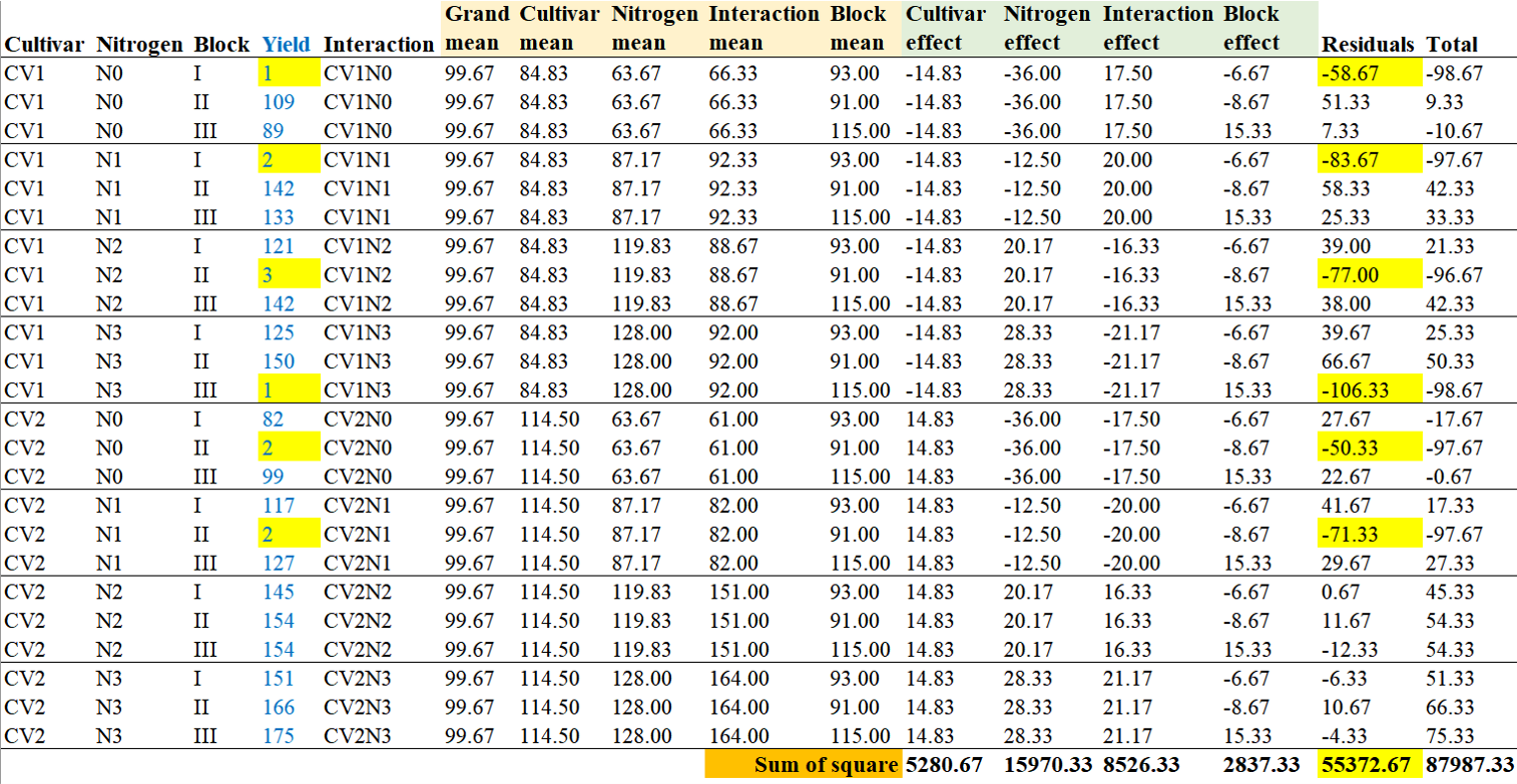
In this scenario, the data would be partitioned as described above, and you can observe a significant increase in the residuals.

---

---

Verify with ANOVA TABLE using R.

Cultivar= rep(c("CV1","CV2"),each=12)
Nitrogen= rep(rep(c("N0","N1","N2","N3"), each=3),2)
Block= rep(c("I","II","III"),8)
Yield= c (99, 109, 89, 115, 142, 133, 121, 157, 142, 125, 150, 139, 82, 104, 99, 117, 125, 127, 145, 154, 154, 151, 166, 175)
dataA= data.frame(Cultivar,Nitrogen,Block,Yield)

ANOVA= aov(Yield~ Cultivar+Nitrogen+Cultivar:Nitrogen+ factor(Block), data=dataA)
summary(ANOVA)

                  Df Sum Sq Mean Sq F value   Pr(>F)    
Cultivar           1    253     253    4.99 0.042327 *  
Nitrogen           3  10695    3565   70.17 1.12e-08 ***
factor(Block)      2   1505     752   14.81 0.000351 ***
Cultivar:Nitrogen  3   1040     347    6.82 0.004604 ** 
Residuals         14    711      51                     
---
Signif. codes:  0 ‘***’ 0.001 ‘**’ 0.01 ‘*’ 0.05 ‘.’ 0.1 ‘ ’ 1

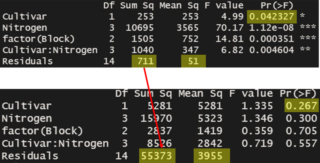
This result is the value verified using R for the calculations we previously performed manually. It matches the values we calculated manually.

Cultivar= rep(c("CV1","CV2"),each=12)
Nitrogen= rep(rep(c("N0","N1","N2","N3"), each=3),2)
Block= rep(c("I","II","III"),8)
Yield= c (1, 109, 89, 2, 142, 133, 121, 3, 142, 125, 150, 1, 82, 2, 99, 117, 2, 127, 145, 154, 154, 151, 166, 175)
dataB= data.frame(Cultivar,Nitrogen,Block,Yield)

ANOVA= aov(Yield~ Cultivar+Nitrogen+Cultivar:Nitrogen+ factor(Block), data=dataB)
summary(ANOVA)

                  Df Sum Sq Mean Sq F value Pr(>F)
Cultivar           1   5281    5281   1.335  0.267
Nitrogen           3  15970    5323   1.346  0.300
factor(Block)      2   2837    1419   0.359  0.705
Cultivar:Nitrogen  3   8526    2842   0.719  0.557
Residuals         14  55373    3955   

Furthermore, this result is the difference that occurs when we assume flooding. In this assumption of flooding, Cultivar does not appear to be significant (p=0.267). This suggests that the differences in yield are not attributed to cultivar variations, but rather considered as errors occurring within the same treatment. As a result, you can observe that the sum of squares for Error has increased from 711.25 to 55372.67.

Using a statistical program can provide results within seconds. However, the important aspect isn’t just knowing how to run a statistical program that yields results in 10 seconds, but understanding the underlying principles within it. Knowing these principles allows you to closely examine your data and understand what might be problematic or insightful.

---

---