How to analyze linear plateau model in R Studio?
# This is the full code to generate the above graph. You can simply copy and paste this code in your R console to obtain the graph.

# to uplopad upload
library (readr)
github= "https://raw.githubusercontent.com/agronomy4future/raw_data_practice/main/sulphur%20application.csv"
dataA=data.frame(read_csv(url(github), show_col_types = FALSE))

# to find reasonable initial values for parameters
fit.lm= lm(yield~sulphur,data=dataA)
a_parameter= fit.lm$coefficients[1]
b_parameter= fit.lm$coefficients[2]
x_mean= mean(dataA$sulphur)

# to define quadratic  plateau function
#a = intercept
#b = slope
#jp = join point or break point

linplat<- function(x, a, b, jp){
  ifelse(x<jp,
         a+b*x,
         a+b*jp)
}

# to find the best fit parameters
library(dplyr)
library(minpack.lm)

model= nlsLM(formula= yield ~ linplat(sulphur, a, b, jp),
             data= dataA,
             start= list(a=a_parameter,
                         b=b_parameter,
                         jp=x_mean))

summary(model)

# to generate a graph
library(ggplot2)
library(minpack.lm)
library(nlraa)

dataA %>%
  ggplot(aes(sulphur, yield)) +
  geom_point(size=4, alpha = 0.5) +
  geom_line(stat="smooth",
            method="nlsLM",
            formula=y~SSlinp(x,a,b,jp),
            se=FALSE,
            color="Dark red") +
  geom_vline(xintercept=23.2722, linetype="solid", color="grey") +
  annotate("text", label=paste("sulphur=","23.3","kg/ha"),
           x=23.3, y=1000, angle=90, hjust=0, vjust=1.5, alpha=0.5)+
  labs(x="Sulphur application (kg/ha)", y="Yield (kg/ha)") +
  theme_grey(base_size=15, base_family="serif")+
  theme(legend.position="none",
        axis.line=element_line(size=0.5, colour="black")) +
  windows(width=5.5, height=5)
When we talk about regression, it’s usually about simple linear regression model. This is about the relationship between two variables.
FYI
□ Simple linear regression (1/5)- correlation and covariance
□ Simple linear regression (2/5)- slope and intercept of linear regression model
Linear plateau model is similar with simple linear model, but linear plateau model is a segmented model, and this statistical model is interested in the critical value (the x-value above which there is no further increase in y), indicating the plateau value (the statistically highest value that y reaches).
I always talk with data. I’ll run the below R code.
library (readr)
github= "https://raw.githubusercontent.com/agronomy4future/raw_data_practice/main/sulphur%20application.csv"
dataA=data.frame(read_csv(url(github), show_col_types= FALSE))
Or you can directly generate the data like below.
variety= rep(c("CV1","CV2","CV3","CV4","CV5"), each=9)
sulphur= c(20.67, 19.9, 19.73,21.16, 21.61, 20.9, 22.36,
            21.97, 21.9, 21.34, 21.28, 21.9, 20.7, 22.65,
            22.16, 22.03, 20.4, 22.47, 22.65, 21.82, 24.41,
            22.34, 24.03, 24.38, 23.6, 23.44, 23.51, 23.89,
            24.7, 22.8, 23.08, 25.05, 24.09, 24.3, 25.23,
            23.14, 24.06, 26.98, 25.71, 23.93, 25.16, 23.79,
            26.34, 24.64, 24.77)
yield= c(1286, 1165, 1176, 1262, 1271, 1221, 1374, 1288,
          1285, 1261, 1281, 1302, 1199, 1368, 1340, 1272,
          1276, 1329, 1361, 1267, 1380, 1386, 1408, 1380,
          1378, 1413, 1400, 1412, 1422, 1381, 1410, 1410,
          1381, 1422, 1389, 1403, 1420, 1403, 1400, 1420,
          1379, 1393, 1417, 1415, 1383)

dataA= data.frame(variety,sulphur,yield)
Also, you can download this data in my Github> https://github.com/agronomy4future/raw_data_practice/blob/main/sulphur%20application.csv
Let’s assume that this data is about yield data in five different crop variety according to different sulphur application. First, this is about analysis for simple linear regression.
library (ggplot2)
ggplot(data=dataA,aes(x=sulphur, y=yield)) +
  geom_smooth(method=lm, level=0.95, se=FALSE, linetype=1, size=0.5, formula= y ~ x) +
  geom_point(aes(shape=variety, fill=variety),col="Black", size=5, stroke = 0.5) +
  scale_shape_manual(values=rep(c(21),5)) +
  scale_fill_manual(values=rep(c("Dark grey"),5))+
  scale_x_continuous(breaks=seq(15,30,5), limits=c(15,30)) +
  scale_y_continuous(breaks=seq(500,1800,300), limits=c(500,1800)) +
  labs(x="sulphur application (kg/ha)", y="Yield (kg/ha)") +
  theme_grey(base_size=15, base_family="serif")+
  theme(legend.position="none",
        axis.line=element_line(size=0.5, colour="black")) +
  windows(width=5.5, height=5)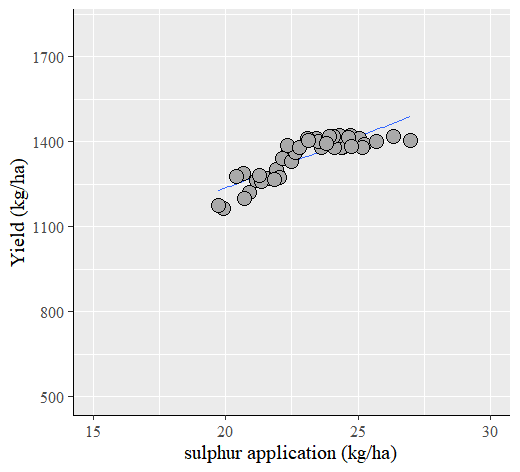
regression= lm (yield~sulphur,data=dataA)
summary(regression)

Call:
lm(formula = yield ~ sulphur, data = dataA)

Residuals:
    Min      1Q  Median      3Q     Max
-85.236 -25.614  -1.877  30.319  64.933

Coefficients:
            Estimate Std. Error t value Pr(>|t|)
(Intercept)  516.204     78.601   6.567 5.46e-08 ***
sulphur       36.028      3.402  10.591 1.47e-13 ***
---
Signif. codes:  0 ‘***’ 0.001 ‘**’ 0.01 ‘*’ 0.05 ‘.’ 0.1 ‘ ’ 1

Residual standard error: 38.79 on 43 degrees of freedom
Multiple R-squared:  0.7229,	Adjusted R-squared:  0.7164
F-statistic: 112.2 on 1 and 43 DF,  p-value: 1.467e-13
We obtained the model equation, y= 516.204 + 36.025x
However, this model equation would be different from actual data because the model equation predicts yield increase when sulphur increases, but in the actual data, yield does not increase at certain point.
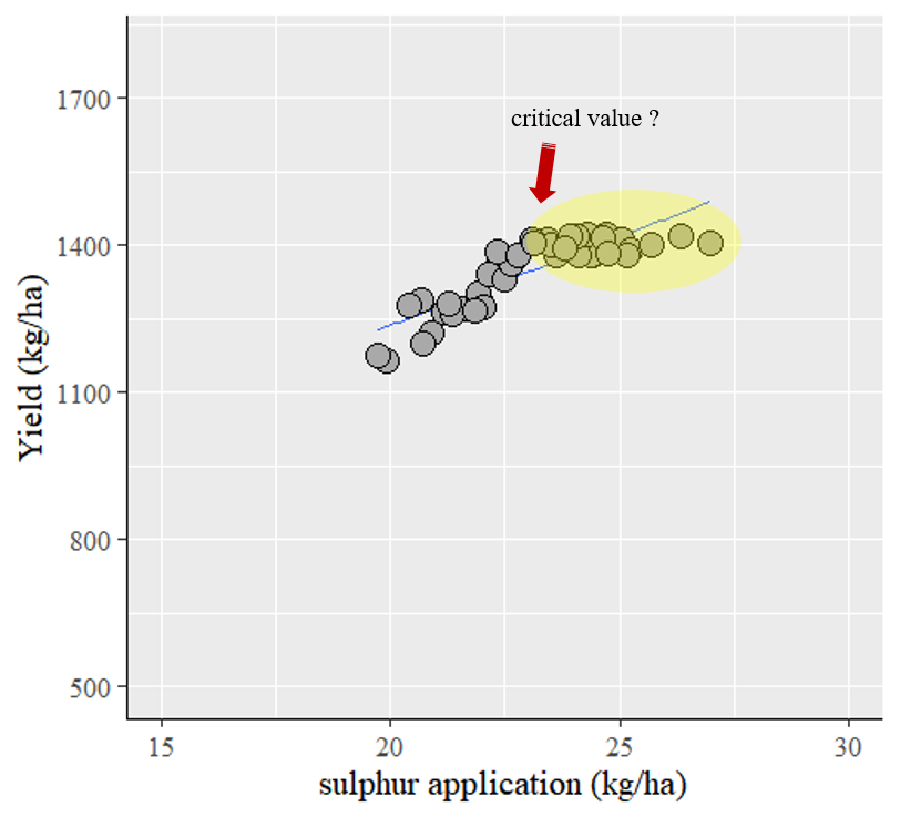
I’m interestedin this certain point. Therefore, I’d like to know the optimun sulphur application to bring about the grestest yield, using a linear plateau model.
1) Find reasonable initial values for parameters
fit.lm= lm(yield~sulphur,data=dataA)
a_parameter= fit.lm$coefficients[1]
b_parameter= fit.lm$coefficients[2]
x_mean= mean(dataA$sulphur)

fit.lm= lm(yield~sulphur,data=dataA)
a_parameter= fit.lm$coefficients[1]
b_parameter= fit.lm$coefficients[2]
x_mean= mean(dataA$sulphur)

> a_parameter
(Intercept)
516.2043

> b_parameter
sulphur
36.02786

> x_mean
23.04378
Now, the gereral values for simple linear regresion were calculated again. a_parameter is for intercept, b_parameter is for slope, and x_mean is for average of sulphur.
2) Define linear plateau function
Linear plateau model was defined as below.
#a = intercept
#b = slope
#jp = join point or break point

linplat= function(x, a, b, jp){
         ifelse(condition= x<jp,
                true= a+b*x,
                false= a+b*jp)
}
“Sometimes, this code causes errors. If an error occurs, you can delete the text identifying the equation.”
linplat= function(x, a, b, jp){
         ifelse(x<jp,
                a+b*x,
                a+b*jp)
}
3) Find best fit parameters
model= nls(yield~linplat(sulphur, a, b, jp),
            data=dataA,
            start=list(a=a_parameter,
                       b=b_parameter,
                       jp=x_mean),
            trace=FALSE,
            nls.control(maxiter=1000))

summary(model)

----------- or -----------

library(minpack.lm)
model= nlsLM(formula= yield ~ linplat(sulphur, a, b, jp),
             data= dataA,
             start=list(a=a_parameter,
                        b=b_parameter,
                        jp=x_mean))

summary(model)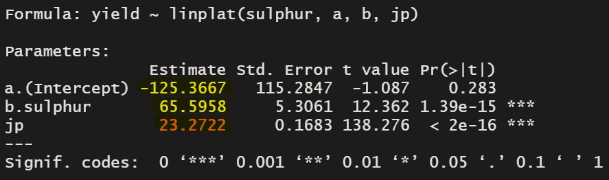
We obtained the linear plateau model equation. The below code is the whole code to obtain this model equation.
# Find reasonable initial values for parameters
fit.lm= lm(yield~sulphur,data=dataA)
a_parameter= fit.lm$coefficients[1]
b_parameter= fit.lm$coefficients[2]
x_mean= mean(dataA$sulphur)

# Define linear plateau function
linplat= function(x, a, b, jp){
         ifelse(x<jp, a+b*x,
         a+b*jp)
}

# Find best fit parameters
library(minpack.lm)
model= nlsLM(formula= yield ~ linplat(sulphur, a, b, jp),
             data= dataA,
             start=list(a=a_parameter,
                         b=b_parameter,
                         jp=x_mean))

summary(model)
Also, we can modify the code as below.
# Find reasonable initial values for parameters
linear <- lm(yield~sulphur, data=dataA)
start_values <- coef(linear)

# Define linear plateau function
linplat<- function(x, a, b, jp){
  ifelse(x<jp, a+b*x,
         a+b*jp)
}

# Find best fit parameters
library(minpack.lm)
model <- nlsLM(formula=yield~linplat(sulphur, a, b, jp),
  data=dataA,
  start=list(
    a=start_values[1],
    b=start_values[2],
    jp=mean(dataA$sulphur)))

summary(model)
Tip!! nlraa() package
install.packages("nlraa")
library(nlraa)
model= nlsLM(formula=yield~SSlinp(sulphur,a,b,jp),data=dataA)
summary(model)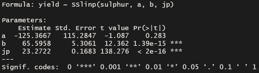
If we use nlraa(), we can obtain the model eqution at once without extra coding. However, it would be better to follow what I suggested step by step to understand the concept of linear plateau model.
How to interpret linear plateau model?
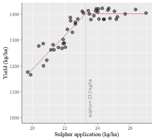
In the model equation; y= – 125.4 + 65.6, the important thing is critical value, 23.3. Statistically, at this point, yield does not increase although sulphur application increases. Therefore, critical value is regarded as the highest value that yield reaches.
Therefore, the model equation is expressed as below.
y= -125.4 + 65.6x if x < 23.3
and when sulphur application is 23.3, yield would be
y= -125.3667 + 65.5958*23.2722 ≈ 1401.2
That is, when 23.3 S kg/ha was applied, yield would be 1,401.2 kg/ha and no more yield increases, indicating the optimum sulphur application would be 23.3 kg/ha.
How to make a graph?
Using the below code, we can easily draw a graph for linear plateau.
dataA %>%
  ggplot(aes(sulphur, yield)) +
  geom_point(size=4, alpha = 0.5) +
  geom_line(stat="smooth",
            method="nlsLM",
            formula=y~SSlinp(x,a,b,jp),
            se=FALSE,
            color="Dark red") +
  labs(x="Sulphur application (kg/ha)", y="Yield (kg/ha)") +
  theme_grey(base_size=15, base_family="serif")+
  theme(legend.position="none",
        axis.line=element_line(size=0.5, colour="black")) +
  windows(width=5.5, height=5)
The breaking point is 23.3 and at this point, yield would be 1,401.2
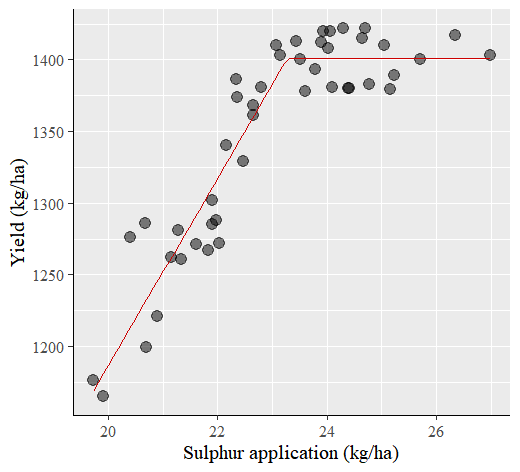
To visualize more clearly, more code will be added.
dataA %>%
  ggplot(aes(sulphur, yield)) +
  geom_point(size=4, alpha = 0.5) +
  geom_line(stat="smooth",
            method="nlsLM",
            formula=y~SSlinp(x,a,b,jp),
            se=FALSE,
            color="Dark red") +
  geom_vline(xintercept=23.2722, linetype="solid", color="grey") +
  annotate("text", label=paste("sulphur=","23.3","kg/ha"),
           x=23.3, y=1000, angle=90, hjust=0, vjust=1.5, alpha=0.5)+
  labs(x="Sulphur application (kg/ha)", y="Yield (kg/ha)") +
  theme_grey(base_size=15, base_family="serif")+
  theme(legend.position="none",
        axis.line=element_line(size=0.5, colour="black")) +
  windows(width=5.5, height=5)
p-value and pseudo R-squared
# Define null model
nullfunct= function(x, m){m}
m.ini= mean(dataA$sulphur)
null= nls(yield~nullfunct(sulphur, m),
          data=dataA,
          start=list(m=m.ini),
          trace=FALSE,
          nls.control(maxiter=1000))

# Find p-value and pseudo R-squared
library(rcompanion)
nagelkerke(model,null)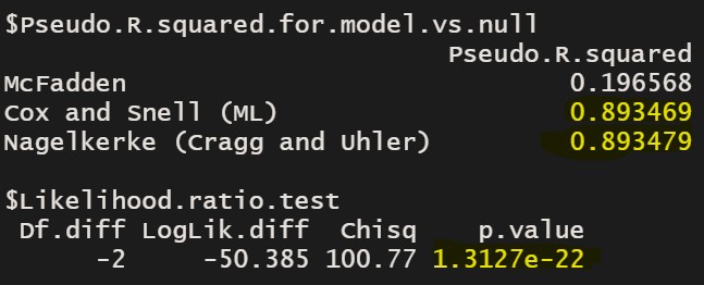
Reference
https://gradcylinder.org/post/linear-plateau/
https://rcompanion.org/handbook/I_11.html
How to analyze the same data as quadratic plateau model? The answer is below.