How to analyze quadratic plateau model in R Studio?
# This is the full code to generate the above graph. You can simply copy and paste this code in your R console to obtain the graph.

# to uplopad data
library(readr)

github="https://raw.githubusercontent.com/agronomy4future/raw_data_practice/main/sulphur%20application.csv"

dataA=data.frame(read_csv(url(github),show_col_types = FALSE))

# to find reasonable initial values for parameters
fit.lm=lm(yield ~ poly(sulphur,2, raw=TRUE),data=dataA)
a_parameter=fit.lm$coefficients[1]
b_parameter=fit.lm$coefficients[2]
c_parameter=fit.lm$coefficients[3]
x_mean=mean(dataA$sulphur)

# to define quadratic  plateau function
# a = intercept
# b = slope
# c = quadratic term (curvy bit)
# jp = join point = break point = critical concentration

qp=function(x, a, b, jp) {
    c=-0.5 * b / jp
    if_else(condition= x < jp,
            true= a + (b * x) + (c * x * x),
            false= a + (b * jp) + (c * jp * jp))
}

# to find the best fit parameters
library(dplyr, warn.conflicts = FALSE)

model=nls(formula=yield ~ qp(sulphur, a, b, jp),
            data=dataA,
            start=list(a=a_parameter, b=b_parameter, jp=x_mean))

summary(model)

# to generate a graph
library(ggplot2)
library(nlraa)
library(minpack.lm)

dataA %>%
  ggplot(aes(sulphur, yield)) +
  geom_point(size=4, alpha = 0.5) +
  geom_line(stat="smooth",
            method="nls",
            formula=y~SSquadp3xs(x,a,b,jp),
            se=FALSE,
            color="Dark red") +
  geom_vline(xintercept=25.0656, linetype="solid", color="grey") +
  annotate("text", label=paste("sulphur=","25.1","kg/ha"),
           x=25.2, y=1000, angle=90, hjust=0, vjust=1.5, alpha=0.5)+
  labs(x="Sulphur application (kg/ha)", y="Yield (kg/ha)") +
  theme_grey(base_size=15, base_family="serif")+
  theme(legend.position="none",
        axis.line=element_line(linewidth=0.5, colour="black")) +
  windows(width=5.5, height=5)
Previous post
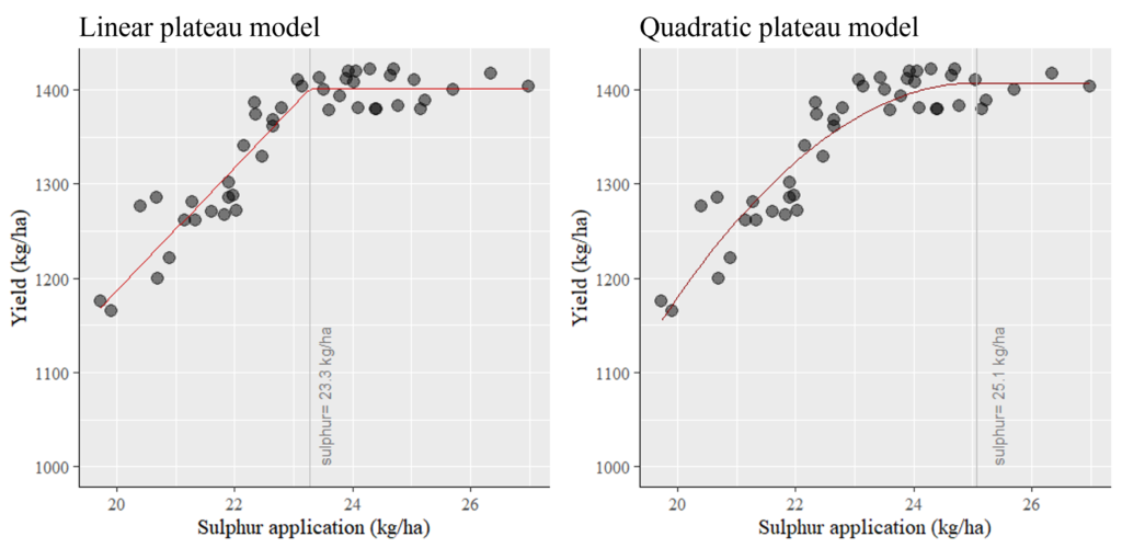
□ How to analyze linear plateau model in R Studio?
In my previous post, I explained how to analyze linear plateau model. I simulated yield data for five different crop varieties with different sulphur applications, and suggsted the optimum sulphur application would be 23.3 kg/ha based on the linear plateau model.
In this time, I’ll explain how to analyze quadratic plateau model with the same data using R studio
1) Data upload
If you run the below code, the data which I simulated will be uploaded to R.
install.packages("readr")
library (readr)

github<- "https://raw.githubusercontent.com/agronomy4future/raw_data_practice/main/sulphur%20application.csv"

dataA<-data.frame(read_csv(url(github)))
Or, you can directly generate data like below.
variety<- rep(c("CV1","CV2","CV3","CV4","CV5"), each=9)
sulphur<- c(20.67, 19.9, 19.73,21.16, 21.61, 20.9, 22.36,
            21.97, 21.9, 21.34, 21.28, 21.9, 20.7, 22.65,
            22.16, 22.03, 20.4, 22.47, 22.65, 21.82, 24.41,
            22.34, 24.03, 24.38, 23.6, 23.44, 23.51, 23.89,
            24.7, 22.8, 23.08, 25.05, 24.09, 24.3, 25.23,
            23.14, 24.06, 26.98, 25.71, 23.93, 25.16, 23.79,
            26.34, 24.64, 24.77)
yield<- c(1286, 1165, 1176, 1262, 1271, 1221, 1374, 1288,
          1285, 1261, 1281, 1302, 1199, 1368, 1340, 1272,
          1276, 1329, 1361, 1267, 1380, 1386, 1408, 1380,
          1378, 1413, 1400, 1412, 1422, 1381, 1410, 1410,
          1381, 1422, 1389, 1403, 1420, 1403, 1400, 1420,
          1379, 1393, 1417, 1415, 1383)

dataA<- data.frame(variety,sulphur,yield)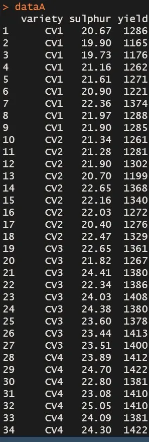
Let’s assume that this data is about yield data for five different crop varieties with different sulphur applications.
2) General quadratic regression model
First of all, I’ll analyze general quadratic regression model.
library (ggplot2)
ggplot(data=dataA,aes(x=sulphur, y=yield)) +
  geom_smooth(method=lm, level=0.95, se=FALSE, linetype=1, size=0.5, formula=y~poly(x,2, raw=TRUE)) +
  geom_point(aes(shape=variety, fill=variety),col="Black", size=5, stroke = 0.5) +
  scale_shape_manual(values=rep(c(21),5)) +
  scale_fill_manual(values=rep(c("Dark grey"),5))+
  scale_x_continuous(breaks=seq(15,30,5), limits=c(15,30)) +
  scale_y_continuous(breaks=seq(500,1800,300), limits=c(500,1800)) +
  labs(x="sulphur application (kg/ha)", y="Yield (kg/ha)") +
  theme_grey(base_size=15, base_family="serif")+
  theme(legend.position="none",
        axis.line=element_line(linewidth=0.5, colour="black")) +
  windows(width=5.5, height=5)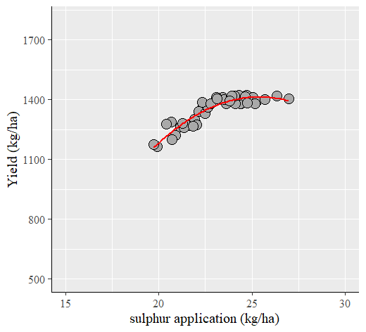
I obtained the graph like above. Now I’ll do statistical analysis for the quadratic regression model.
regression<- lm(yield ~ poly(sulphur,2, raw=TRUE), data=dataA)
summary(regression)
anova(regression)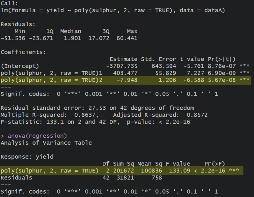
It shows the quadratic term is significant, and also regression variance is significant. Therefore, I can suggest the model equation; y= -3707.735 + 403.4772 - 7.948x2.
Now, I’d like to find the optimum sulphur amount to bring about the greatest yield. Simply we can ‘predict’ according to the model equation, but I’d like to know the critical value as a break point (the x-value above which there is no further increase in y), indicating the ‘plateau value’ (the statistically highest value that y reaches) as quadratic regression model. This is called ‘Quadratic plateau model.’
3) Quadratic plateau model
Now, I’ll introdue how to analyze quadratic plateau model in R step by step.
3.1) to find reasonable initial values for parameters
fit.lm<-lm(yield ~ poly(sulphur,2, raw=TRUE),data=dataA)
a_parameter<-fit.lm$coefficients[1]
b_parameter<-fit.lm$coefficients[2]
c_parameter<-fit.lm$coefficients[3]
x_mean<-mean(dataA$sulphur)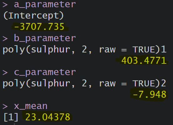
Now, the gereral values for quadratic regresion were calculated again. a_parameter is for intercept, b_parameter is for slope x, c_parameter is for slope x2, and x_mean is for average of sulphur. These values are the same as model equation, y= -3707.735 + 403.4772 - 7.948x2
3.2) to define quadratic plateau function
Quadratic plateau model is defined as below.
# a = intercept
# b = slope
# c = quadratic term (curvy bit)
# jp = join point = break point

qp <- function(x, a, b, jp) {
    c <- -0.5 * b / jp
    if_else(condition = x < jp,
            true  = a + (b * x) + (c * x * x),
            false = a + (b * jp) + (c * jp * jp))
}
FYI, this is the definition of linear plateau model.
#a = intercept
#b = slope
#jp = join point or break point

linplat<- function(x, a, b, jp){
  ifelse(x<jp, a+b*x,
         a+b*jp)
}
3.3) to find the best fit parameters
library(dplyr)
model <- nls(formula=yield ~ qp(sulphur, a, b, jp),
            data=dataA,
            start=list(a=a_parameter, b=b_parameter, jp=x_mean))

summary(model)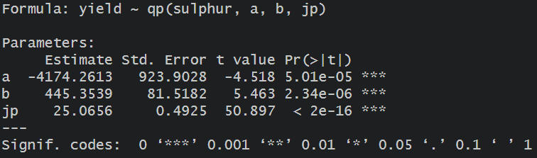
I obtained the quadratic plateau model equation.
y≈ -4174.26 + 445.35x + __x2.
This code does not provide quadratic parameter, but simply we can calculate by hand.
c= -0.5 * b / jp
c= -0.5 * 445.3539 / 25.0656 ≈ -8.88
and critical value is 25.0656. Then, quadratic plateau model would be written as
y≈ -4174.26 + 445.35x -8.88x2 (if x < 25.1)
This is another code to find the best fit parameters
quadratic<-lm(yield~poly(sulphur,2,raw = TRUE), data=dataA)
parameter<-coef(quadratic)

model<- nls(formula=yield~qp(sulphur, a, b, jp),
            data=dataA,
            start=list(a=parameter[1],
                       b=parameter[2],
                       jp=mean(dataA$sulphur)))

summary(model)

----------- or -----------

library(minpack.lm)
model <- nlsLM(formula=yield~qp(sulphur, a, b, jp),
              data=dataA,
              start=list(a=a_parameter,
                         b=b_parameter,
                         jp=x_mean))

summary(model)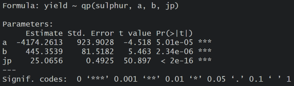
If you use nlraa() package, you can obtain the model eqution at once without extra coding. However, it would be better to follow what I suggested step by step to understand the concept of quadratic plateau model.
install.packages("nlraa")
library(nlraa)
model<-nlsLM(formula=yield~SSquadp3xs(sulphur,a,b,jp),
       data=dataA)
summary(model)
3.4) to generate a graph
library(ggplot2)
library(minpack.lm)
library(nlraa)

dataA %>%
  ggplot(aes(sulphur, yield)) +
  geom_point(size=4, alpha = 0.5) +
  geom_line(stat="smooth",
            method="nls",
            formula=y ~ SSquadp3xs(x, a, b, jp),
            se=FALSE,
            color="Dark red") +
  labs(x="Sulphur application (kg/ha)", y="Yield (kg/ha)") +
  theme_grey(base_size=15, base_family="serif")+
  theme(legend.position="none",
        axis.line=element_line(linewidth=0.5, colour="black")) +
  windows(width=5.5, height=5)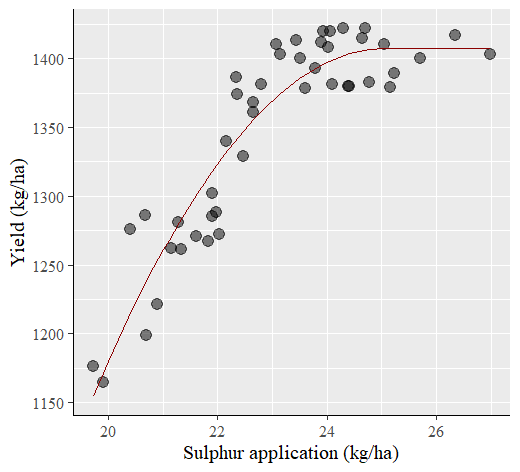
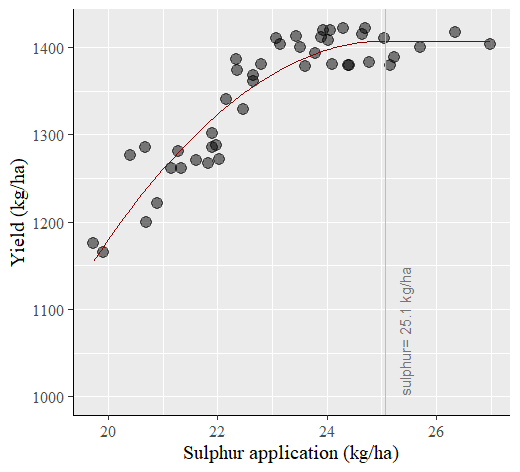
The breaking point is 25.1 and at this point, yield would be 1,410 according to the model equation, y≈ -4174.26 + 445.35x -8.88x2 (if x < 25.1).
To visualize more clearly, more code will be added.
dataA %>%
  ggplot(aes(sulphur, yield)) +
  geom_point(size=4, alpha = 0.5) +
  geom_line(stat="smooth",
            method="nlsLM",
            formula=y~SSquadp3xs(x,a,b,jp),
            se=FALSE,
            color="Dark red") +
  geom_vline(xintercept=25.0656, linetype="solid", color="grey") +
  annotate("text", label=paste("sulphur=","25.1","kg/ha"),
           x=25.2, y=1000, angle=90, hjust=0, vjust=1.5, alpha=0.5)+
  labs(x="Sulphur application (kg/ha)", y="Yield (kg/ha)") +
  theme_grey(base_size=15, base_family="serif")+
  theme(legend.position="none",
        axis.line=element_line(linewidth=0.5, colour="black")) +
  windows(width=5.5, height=5)
3.5) How to interpret quadratic plateau model?
y≈ -4174.26 + 445.35x -8.88x2 (if x < 25.1)
In the model equation; y≈ -4174.26 + 445.35x -8.88x2 (if x < 25.1), the important thing is critical value, 25.1. Statistically, at this point, yield does not increase although sulphur application increases. Therefore, critical value is regarded as the highest value that yield reaches.
and when sulphur application is 25.1, yield would be
y≈ -4174.26 + 445.35*25.0656 – 8.88*25.0656^2 ≈ 1409.5
That is, when 25.1 S kg/ha was applied, yield would be 1409.5 kg/ha and no more yield increases, indicating the optimum sulphur application would be 25.1 kg/ha.
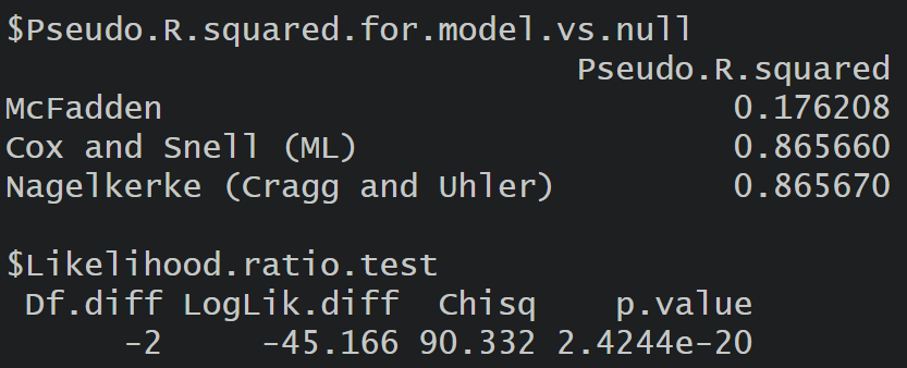
4) p-value and pseudo R-squared
nullfunct<-function(x, m){m}
m.ini<-mean(dataA$yield)
null<-nls(yield~nullfunct(sulphur, m),
           data=dataA,
           start=list(m=m.ini),
           trace=FALSE,
           nls.control(maxiter = 1000))

library(rcompanion)
nagelkerke(model, null)