---

Before diving into in-depth data analysis, a crucial step is data preprocessing. This essential process not only ensures better data quality but also significantly improves the efficiency of your analysis. In this guide, I will introduce a range of powerful Python methods for data preprocessing, equipping you with the tools to optimize your data for more accurate and insightful analysis.

I use Goolge Colab when using Python because it’s more user friendly. Please refer how to setup Google Colab in below post.

---

□ How to use Google Colab for Python (power tool to analyze data)?

---

First, let’s mount your Google Colab environment.

To do this, use the following code:

from google.colab import drive drive.mount('/content/drive')

Next, let’s proceed to import the data. I have uploaded a dataset to my GitHub repository. By copying and pasting the code snippet below, you can automatically download the data.”

import pandas as pd

url="https://raw.githubusercontent.com/agronomy4future/raw_data_practice/main/python_practice.csv"

dataA=pd.read_csv(url)

Next, let’s see how the data is organized. First, I’ll see the top 15 rows.

print(dataA.head(15))

  genotype  height  spike_weight  disease_spot heat_tolerance      region 
0       CV1    86.5         27.90             0            yes    Mid_East   
1       CV2    85.5         33.77             1             no  Test_field   
2       CV2    95.5         33.00             3             no  Test_field   
3       CV2   100.5         22.71             0             no       North   
4       CV2    99.5         28.88             0             no       North   
5       CV1    98.5         25.74             0             no  Test_field   
6       CV1   113.5         33.44             1             no  Test_field   
7       CV1   104.5         27.74             3             no       North   
8       CV2   104.5         29.83             2             no    Mid_West   
9       CV1   127.5         25.84             0             no       North   
10      CV2    92.5         26.22             0             no    Mid_West   
11      CV1   129.5         26.29             0            yes  Test_field   
12      CV2    90.5         34.40             0             no    Mid_East   
13      CV1   123.5         39.82             0             no  Test_field   
14      CV2    94.5           NaN             0            yes  Test_field   

          yield  
0   16861.42400  
1    1702.05230  
2    4425.96200  
3   21960.97061  
4    3843.35520  
5    3733.12160  
6    8217.08960  
7    7258.00560  
8    6382.91070  
9   28899.63692  
10   2697.82080  
11  27785.22510  
12   1803.34300  
13  11067.21780  
14  39588.25770  

Additionally, let’s check the number of rows and columns in this data, identify any duplicated entries, and resolve them by keeping one and removing the others.”

# to check the number of rows and columns
print(dataA.shape)
> (1338, 7)

# to see how many duplicated data exist
print("duplicated data No.", len(dataA[dataA.duplicated()]))
> duplicated data No. 1

# to see what the duplicated data are
print(dataA[dataA.duplicated(keep=False)].sort_values(by=list(dataA.columns)).head())
genotype  height  spike_weight  disease_spot heat_tolerance region  
195       CV2      86.5         30.59        0              no North   
581       CV2      86.5         30.59        0              no North   

     yield  
195  1616.0631  
581  1616.0631  

# to keep one and removing the others.
dataA.drop_duplicates(inplace=True, keep="first", ignore_index=True)

Now, I’ll examine the structure of this data.

print(dataA.info())

<class 'pandas.core.frame.DataFrame'>
RangeIndex: 1337 entries, 0 to 1336
Data columns (total 7 columns):
 #   Column          Non-Null Count  Dtype  
---  ------          --------------  -----  
 0   genotype        1337 non-null   object 
 1   height          1337 non-null   float64
 2   spike_weight    1332 non-null   float64
 3   disease_spot    1337 non-null   int64  
 4   heat_tolerance  1337 non-null   object 
 5   region          1337 non-null   object 
 6   yield           1337 non-null   float64
dtypes: float64(3), int64(1), object(3)

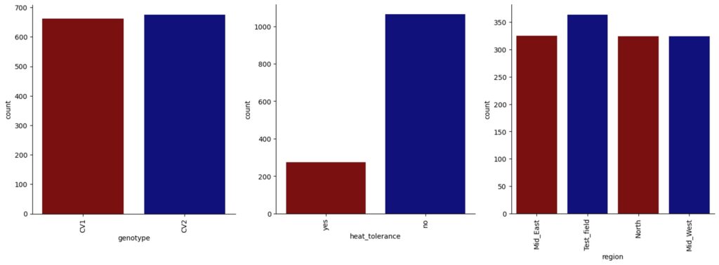
I’ll create a graph to visualize the number of categorical values.

import seaborn as sns
import matplotlib.pyplot as plt

custom_palette = ["darkred", "darkblue"]

for col in dataA.select_dtypes(include=['object', 'category']).columns:
fig = sns.catplot(x=col, kind="count", data=dataA, hue=None, palette=custom_palette)
fig.set_xticklabels(rotation=90)
plt.show() 

python_code/data_check_process.ipynb at main · agronomy4future/python_code (github.com)

---