Performing Regression Analysis in R with Variables in the Same Column
When analyzing regression, we typically assume that two continuous variables are situated in separate columns, allowing us to easily designate them as x and y. However, in many cases, data is organized vertically, and variables of interest are found within the same column. This vertical structuring is, in fact, the fundamental data arrangement when conducting data analysis.
Now, let’s delve further into the discussion by examining the dataset. Let’s proceed by uploading the dataset.”
library(readr)
github="https://raw.githubusercontent.com/agronomy4future/raw_data_practice/main/wheat_grain_Fe_uptake.csv"
dataA= data.frame(read_csv(url(github), show_col_types= FALSE))

dataA
      Location Season Genotype Reps Iron_ton_ha      Stage   Fe
1       East   2021      CV1    1     21.7127   Vegetative  0.44
2       East   2021      CV1    2      8.7340   Vegetative  0.30
3       East   2021      CV1    3      9.5003   Vegetative  0.31
4       East   2021      CV1    4      5.9481   Vegetative  0.37
5       East   2021      CV1    5      7.4608   Vegetative  0.30
6       East   2021      CV1    6     20.5326   Vegetative  0.33
7       East   2021      CV1    7     19.8532   Vegetative  0.29
8       East   2021      CV1    8      7.9718   Vegetative  0.35
9       East   2021      CV1    9     15.0087   Vegetative  0.38
10      East   2021      CV1   10      5.6608   Vegetative  0.40
.
.
.

str(dataA)
'data.frame':	2814 obs. of  7 variables:
 $ Location   : chr  "East" "East" "East" "East" ...
 $ Season     : num  2021 2021 2021 2021 2021 ...
 $ Genotype   : chr  "CV9" "CV9" "CV9" "CV9" ...
 $ Reps       : num  1 2 3 4 5 6 7 8 9 10 ...
 $ Iron_ton_ha: num  7.58 4.12 3.09 7.43 11.48 ...
 $ Stage      : chr  "Vegetative" "Vegetative" "Vegetative" "Vegetative" ...
 $ Fe         : num  0.36 0.32 0.39 0.37 0.36 0.36 0.32 0.33 0.37 0.33 ...
This data pertains to iron content in both wheat grains and soil at three different growing stages for 9 different genotypes in two locations (East and North) across two seasons.
Let’s examine this data structure. Categorical variables—Location, Season, Genotype, and Stage—are organized in columns. Now, suppose I want to analyze the regression between the 2021 and 2022 seasons across genotypes concerning the Fe at maturity. Would I need to copy the 2022 season data and paste it next to the 2021 data? While this approach is manageable for small datasets, it becomes cumbersome with larger datasets.
Today, I’ll introduce a method for analyzing regression when variables are in the same column. I’ll use the following code.
library(dplyr)
library(tidyr)

dataB= dataA %>%
  group_by(Location, Season, Genotype, Stage) %>%
  summarise(Iron_ton_ha=list(Iron_ton_ha), Fe=list(Fe)) %>%
  pivot_wider(names_from=Season, values_from=c(Iron_ton_ha, Fe), names_sep="_") %>%
  unnest(everything())

Error in `unnest()`:
! In row 1, can't recycle input of size 20 to size 19.
Here, I found one problem. The data cannot be summarized due to different row number. Let’s check the row number.
data.frame(dataA %>%
  group_by(Location, Season, Genotype, Stage) %>%
  summarise(count = n()))

    Location Season Genotype        Stage count
1       East   2021      CV1     Maturity    20
2       East   2021      CV1 Reproductive    20
3       East   2021      CV1   Vegetative    20
4       East   2021     CV10     Maturity    20
5       East   2021     CV10 Reproductive    20
6       East   2021     CV10   Vegetative    20
7       East   2021     CV11     Maturity    20
8       East   2021     CV11 Reproductive    20
9       East   2021     CV11   Vegetative    20
10      East   2021     CV12     Maturity    10
11      East   2021     CV12 Reproductive    10
12      East   2021     CV12   Vegetative    10
13      East   2021      CV2     Maturity    20
.
.
.
Now I see some data does not have 20 rows as the basic replicates. Let’s filter data which has not 20 replicates.
filtered_data= data.frame(dataA %>%
group_by(Location, Season, Genotype, Stage) %>%
summarise(count= n()) %>%
filter(count!= 20))
Location Season Genotype Stage count
1 East 2021 CV12 Maturity 10
2 East 2021 CV12 Reproductive 10
3 East 2021 CV12 Vegetative 10
4 East 2021 CV3 Maturity 19
5 East 2021 CV3 Reproductive 19
6 East 2021 CV3 Vegetative 19
7 East 2022 CV1 Maturity 19
8 East 2022 CV1 Reproductive 19
9 East 2022 CV1 Vegetative 19
10 East 2022 CV12 Maturity 10
11 East 2022 CV12 Reproductive 10
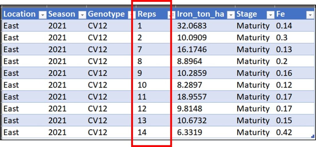
12 East 2022 CV12 Vegetative 10Let’s check this data in Excel. For example, At East in 2021 season for CV12 does not have 20 replicates. So, when the row number is not the same, it would not be possible to use pivot_wider().
I will introduce two methods to solve this problem.
1) to delete data that does not have 20 replicates
First, I will delete data that does not have 20 replicates using the following code.
library(dplyr)

dataA_filtered= dataA %>%
  group_by(Location, Season, Genotype, Stage) %>%
  filter(n()==20) %>%
  ungroup()
After removing data with fewer than 20 replicates, I will then provide a summary.
dataB= dataA_filtered %>%
  group_by(Location, Season, Genotype, Stage) %>%
  summarise(Iron_ton_ha=list(Iron_ton_ha), Fe=list(Fe)) %>%
  pivot_wider(names_from=Season, values_from=c(Iron_ton_ha, Fe), names_sep="_") %>%
  unnest(everything())

dataB
    Location Genotype     Stage    Iron_ton_ha_2021 Iron_ton_ha_2022 Fe_2021 Fe_2022
1       East      CV1     Maturity      21.7127            NA        0.13      NA
2       East      CV1     Maturity      8.7340             NA        0.14      NA
3       East      CV1     Maturity      9.5003             NA        0.12      NA
4       East      CV1     Maturity      5.9481             NA        0.18      NA
5       East      CV1     Maturity      7.4608             NA        0.12      NA
6       East      CV1     Maturity      20.5326            NA        0.24      NA
7       East      CV1     Maturity      19.8532            NA        0.21      NA
8       East      CV1     Maturity      7.9718             NA        0.17      NA
9       East      CV1     Maturity      15.0087            NA        0.32      NA
10      East      CV1     Maturity      5.6608             NA        0.14      NA
.
.
.
2) to add dummy rows
Second, we can add dummy rows to align the data to have 20 rows.
library(dplyr)
library(tidyr)

# Filter data with at least 20 replicates
dataA_filtered= dataA %>%
  group_by(Location, Season, Genotype, Stage) %>%
  filter(n()>=20) %>%
  ungroup()

# Add dummy rows to reach 20 replicates for each group
dummy_rows= dataA_filtered %>%
            complete(Location, Season, Genotype, Stage,
            fill = list(Iron_ton_ha=NA, Fe=NA))

# Combine original data and dummy rows
dataA_combined= bind_rows(dataA_filtered, dummy_rows)

# Create dataB with summary
dataB= dataA_filtered %>%
  group_by(Location, Season, Genotype, Stage) %>%
  summarise(Iron_ton_ha=list(Iron_ton_ha), Fe=list(Fe)) %>%
  pivot_wider(names_from=Season, values_from=c(Iron_ton_ha, Fe), names_sep="_") %>%
  unnest(everything())

dataB
    Location Genotype Stage    Iron_ton_ha_2021  Iron_ton_ha_2022  Fe_2021  Fe_2022
1   East      CV1     Maturity   21.7127          NA               0.13      NA
2   East      CV1     Maturity   8.7340           NA               0.14      NA
3   East      CV1     Maturity   9.5003           NA               0.12      NA
4   East      CV1     Maturity   5.9481           NA               0.18      NA
5   East      CV1     Maturity   7.4608           NA               0.12      NA
6   East      CV1     Maturity   20.5326          NA               0.24      NA
7   East      CV1     Maturity   19.8532          NA               0.21      NA
8   East      CV1     Maturity   7.9718           NA               0.17      NA
9   East      CV1     Maturity   15.0087          NA               0.32      NA
10  East      CV1     Maturity   5.6608           NA               0.14      NA
.
.
.
Finally, I transformed the data structure as follows:
      Location Season Genotype Reps Iron_ton_ha      Stage   Fe
1       East   2021      CV1    1     21.7127   Vegetative  0.44
2       East   2021      CV1    2      8.7340   Vegetative  0.30
3       East   2021      CV1    3      9.5003   Vegetative  0.31
4       East   2021      CV1    4      5.9481   Vegetative  0.37
5       East   2021      CV1    5      7.4608   Vegetative  0.30
6       East   2021      CV1    6     20.5326   Vegetative  0.33
7       East   2021      CV1    7     19.8532   Vegetative  0.29
8       East   2021      CV1    8      7.9718   Vegetative  0.35
9       East   2021      CV1    9     15.0087   Vegetative  0.38
10      East   2021      CV1   10      5.6608   Vegetative  0.40
.
.
.
                                   ↓
                                   ↓
    Location Genotype Stage    Iron_ton_ha_2021  Iron_ton_ha_2022  Fe_2021  Fe_2022
1   East      CV1     Maturity   21.7127          NA                0.13      NA
2   East      CV1     Maturity   8.7340           NA                0.14      NA
3   East      CV1     Maturity   9.5003           NA                0.12      NA
4   East      CV1     Maturity   5.9481           NA                0.18      NA
5   East      CV1     Maturity   7.4608           NA                0.12      NA
6   East      CV1     Maturity   20.5326          NA                0.24      NA
7   East      CV1     Maturity   19.8532          NA                0.21      NA
8   East      CV1     Maturity   7.9718           NA                0.17      NA
9   East      CV1     Maturity   15.0087          NA                0.32      NA
10  East      CV1     Maturity   5.6608           NA                0.14      NA
.
.
.
Now, let’s analyze regression. However, this is raw data. So, I’ll summarize data to provide mean and standard error. In the introducton, I said I want to analyze the regression between the 2021 and 2022 seasons across genotypes concerning the FeFe
library(dplyr)
dataC= data.frame(dataB %>%
                  group_by(Location, Genotype, Stage) %>%
                  dplyr::summarize(across(c(Fe_2021, Fe_2022),
                                            .fns= list(Mean=mean,
                                             SD= sd,
                                             n=length,
                                             se=~ sd(.)/sqrt(length(.))))))
And I’ll only select mean and standard error columns, and change the column name to simplify data.
dataC=dataC[, c("Location", "Genotype", "Stage", "Fe_2021_Mean",
"Fe_2021_se", "Fe_2022_Mean", "Fe_2022_se")]
dataC
Location Genotype Stage Fe_2021_Mean Fe_2021_se Fe_2022_Mean Fe_2022_se
1 East CV1 Maturity 0.1565 0.012036676 NA NA
2 East CV1 Reproductive 0.3130 0.004594046 NA NA
3 East CV1 Vegetative 0.3585 0.011292172 NA NA
4 East CV10 Maturity 0.0955 0.008158786 0.0485 0.003101358
5 East CV10 Reproductive 0.2700 0.007914012 0.2285 0.006167615
6 East CV10 Vegetative 0.3730 0.008463544 0.2630 0.007646809
7 East CV11 Maturity 0.1785 0.018768324 0.0405 0.002457534
8 East CV11 Reproductive 0.3145 0.006548403 0.2380 0.005553567
9 East CV11 Vegetative 0.3810 0.018791095 0.2945 0.003661679
10 East CV2 Maturity 0.1490 0.012853425 0.0525 0.001601808
11 East CV2 Reproductive 0.2915 0.005092564 0.2320 0.007595012
12 East CV2 Vegetative 0.3500 0.020938506 0.2870 0.005577209
13 East CV3 Maturity NA NA 0.0520 0.002575185
14 East CV3 Reproductive NA NA 0.2335 0.004369451
15 East CV3 Vegetative NA NA 0.2915 0.010266835
16 East CV4 Maturity 0.1580 0.013564660 0.0525 0.001758438
17 East CV4 Reproductive 0.3175 0.016106145 0.2355 0.005870309
18 East CV4 Vegetative 0.3850 0.009472953 0.3385 0.007923151
19 East CV5 Maturity 0.1640 0.019939382 0.0515 0.001817314
20 East CV5 Reproductive 0.3270 0.008049191 0.2325 0.006235510
21 East CV5 Vegetative 0.3810 0.011376337 0.3105 0.009799973
22 East CV6 Maturity 0.1710 0.019027681 0.0500 0.003402785
23 East CV6 Reproductive 0.3140 0.009824781 0.2180 0.006712126
24 East CV6 Vegetative 0.3655 0.012171472 0.2650 0.008475972
25 East CV7 Maturity 0.1560 0.015583392 0.0590 0.001762176
26 East CV7 Reproductive 0.3190 0.005021008 0.2290 0.005520297
27 East CV7 Vegetative 0.3680 0.012723786 0.2730 0.008146682
28 East CV8 Maturity 0.1760 0.016676488 0.0580 0.003043544
29 East CV8 Reproductive 0.3160 0.006897749 0.2330 0.005186014
30 East CV8 Vegetative 0.3700 0.009814061 0.2765 0.006418518
31 East CV9 Maturity 0.1205 0.011731088 0.0595 0.008061442
32 East CV9 Reproductive 0.2925 0.008074489 0.2275 0.004345294
33 East CV9 Vegetative 0.3575 0.004345294 0.2660 0.007588079
34 North CV1 Maturity 0.1090 0.012771267 0.0645 0.004728135
35 North CV1 Reproductive 0.2455 0.009664776 0.2640 0.007448066
36 North CV1 Vegetative 0.4655 0.010772162 0.2915 0.007118360
37 North CV10 Maturity 0.0930 0.009870210 0.0480 0.002675424
38 North CV10 Reproductive 0.2515 0.005092564 0.2375 0.005225192
39 North CV10 Vegetative 0.4125 0.008792192 0.2505 0.007762087
40 North CV11 Maturity 0.1070 0.013651682 0.0565 0.002926737
41 North CV11 Reproductive 0.2650 0.009104655 0.2730 0.005083513
42 North CV11 Vegetative 0.4620 0.009222398 0.2960 0.010036774
43 North CV12 Maturity 0.1335 0.017818899 0.0680 0.004448536
44 North CV12 Reproductive 0.2660 0.005399805 0.2525 0.006722899
45 North CV12 Vegetative 0.4625 0.009144311 0.2610 0.007843871
46 North CV2 Maturity 0.1790 0.017151032 0.0490 0.002605662
47 North CV2 Reproductive 0.2925 0.005019698 0.2520 0.007595012
48 North CV2 Vegetative 0.4590 0.010635096 0.2765 0.005861336
49 North CV3 Maturity 0.1205 0.009773083 0.0545 0.003661679
50 North CV3 Reproductive 0.2665 0.005245299 0.2395 0.005779956
51 North CV3 Vegetative 0.4745 0.010893624 0.2630 0.005942709
52 North CV4 Maturity NA NA NA NA
53 North CV4 Reproductive 0.3065 0.006418518 0.2420 0.005553567
54 North CV4 Vegetative 0.4830 0.008146682 0.2560 0.005201214
55 North CV5 Maturity 0.1055 0.008254983 0.0660 0.004888224
56 North CV5 Reproductive 0.2660 0.005911630 0.2470 0.006653056
57 North CV5 Vegetative 0.4615 0.011904776 NA NA
58 North CV6 Maturity 0.1510 0.028106002 0.0540 0.002937955
59 North CV6 Reproductive 0.2870 0.004925765 0.2355 0.004892260
60 North CV6 Vegetative 0.4755 0.011013747 NA NA
61 North CV7 Maturity 0.2160 0.028045076 NA NA
62 North CV7 Reproductive 0.2885 0.006854695 0.2410 0.004861232
63 North CV7 Vegetative 0.4555 0.016709200 0.2570 0.010389772
64 North CV8 Maturity 0.1665 0.018935833 0.0495 0.002944665
65 North CV8 Reproductive 0.2940 0.005730803 0.2510 0.002800376
66 North CV8 Vegetative 0.4520 0.008447983 0.2805 0.008567841
67 North CV9 Maturity 0.1255 0.012762507 NA NA
68 North CV9 Reproductive 0.2590 0.007104483 0.2495 0.004441135
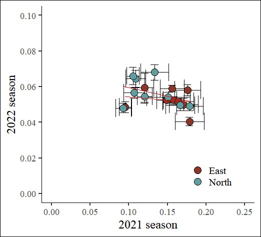
69 North CV9 Vegetative 0.4100 0.009090191 0.2525 0.009729905I’ll create a regression graph.
library(ggplot2)
FIGA=ggplot(data=subset(dataC, Stage=="Maturity"), aes(x=Fe_2021_Mean, y=Fe_2022_Mean)) +

  geom_errorbar(aes(xmin=Fe_2021_Mean-Fe_2021_se, xmax=Fe_2021_Mean+Fe_2021_se),
                position=position_dodge(0.7),
                width=0.01) +
  geom_errorbar(aes(ymin=Fe_2022_Mean-Fe_2022_se, ymax=Fe_2022_Mean+Fe_2022_se),
                position=position_dodge(0.7),
                width=0.01) +

  geom_point(aes(fill=Location, shape=Location), color= "black", size = 5) +
  geom_smooth(aes(group=Location),method='lm', linetype=1, se=FALSE, color="red", formula=y~x, size=0.5) +

  scale_fill_manual(values=c("tomato4","cadetblue")) +
  scale_shape_manual(values=c(21,21)) +
  scale_x_continuous(breaks=seq(0,0.25,0.05),limits=c(0,0.25)) +
  scale_y_continuous(breaks=seq(0,0.1,0.02),limits=c(0,0.1)) +
  labs(x="2021 season", y="2022 season") +
  theme_classic(base_size=18, base_family="serif") +
  theme(legend.position=c(0.8,0.15),
        legend.title=element_blank(),
        legend.key=element_rect(color="white", fill="white"),
        legend.text=element_text(family="serif", face="plain",
                                 size=15, color="black"),
        legend.background= element_rect(fill="white"),
        strip.background=element_rect(color="white",
                                      size=0.5, linetype="solid"),
        axis.line = element_line(linewidth = 0.5, colour="black"))
FIGA+windows(width=5.5, height=5)
When using Excel, we have to move data one by one when analyzing regression. In contrast, this R code simply transposes the data structure, making it easy for us to analyze the data.
This is the full code;
https://github.com/agronomy4future/r_code/blob/main/regression_analysis_with_variables_in_the_same_column
library(readr)
library(dplyr)
library(tidyr)
library(ggplot2)

# data upload
github="https://raw.githubusercontent.com/agronomy4future/raw_data_practice/main/wheat_grain_Fe_uptake.csv"
dataA= data.frame(read_csv(url(github), show_col_types= FALSE))

# to adjust unbalanced data
dataA_filtered= dataA %>%
  group_by(Location, Season, Genotype, Stage) %>%
  filter(n()>=20) %>%
  ungroup()

dummy_rows= dataA_filtered %>%
  complete(Location, Season, Genotype, Stage,
           fill = list(Iron_ton_ha=NA, Fe=NA))

dataA_combined= bind_rows(dataA_filtered, dummy_rows)

# to transpose data structure
dataB= dataA_filtered %>%
  group_by(Location, Season, Genotype, Stage) %>%
  summarise(Iron_ton_ha=list(Iron_ton_ha), Fe=list(Fe)) %>%
  pivot_wider(names_from=Season, values_from=c(Iron_ton_ha, Fe), names_sep="_") %>%
  unnest(everything())

# to summarize data
dataC= data.frame(dataB %>%
                  group_by(Location, Genotype, Stage) %>%
                  dplyr::summarize(across(c(Fe_2021, Fe_2022),
                                            .fns= list(Mean=mean,
                                             SD= sd,
                                             n=length,
                                             se=~ sd(.)/sqrt(length(.))))))

# to simplify data
dataC=dataC[, c("Location", "Genotype", "Stage", "Fe_2021_Mean",
                "Fe_2021_se", "Fe_2022_Mean", "Fe_2022_se")]

# to create a graph
FIGA=ggplot(data=subset(dataC, Stage=="Maturity"), aes(x=Fe_2021_Mean, y=Fe_2022_Mean)) +

  geom_errorbar(aes(xmin=Fe_2021_Mean-Fe_2021_se, xmax=Fe_2021_Mean+Fe_2021_se),
                position=position_dodge(0.7),
                width=0.01) +
  geom_errorbar(aes(ymin=Fe_2022_Mean-Fe_2022_se, ymax=Fe_2022_Mean+Fe_2022_se),
                position=position_dodge(0.7),
                width=0.01) +

  geom_point(aes(fill=Location, shape=Location), color= "black", size = 5) +
  geom_smooth(aes(group=Location),method='lm', linetype=1, se=FALSE, color="red", formula=y~x, size=0.5) +

  scale_fill_manual(values=c("tomato4","cadetblue")) +
  scale_shape_manual(values=c(21,21)) +
  scale_x_continuous(breaks=seq(0,0.25,0.05),limits=c(0,0.25)) +
  scale_y_continuous(breaks=seq(0,0.1,0.02),limits=c(0,0.1)) +
  labs(x="2021 season", y="2022 season") +
  theme_classic(base_size=18, base_family="serif") +
  theme(legend.position=c(0.8,0.15),
        legend.title=element_blank(),
        legend.key=element_rect(color="white", fill="white"),
        legend.text=element_text(family="serif", face="plain",
                                 size=15, color="black"),
        legend.background= element_rect(fill="white"),
        strip.background=element_rect(color="white",
                                      linewidth=0.5, linetype="solid"),
        axis.line = element_line(linewidth = 0.5, colour="black"))
FIGA+windows(width=5.5, height=5)