Understanding Mean Absolute Error (MAE) in ANOVA: A Step-by-Step Guide to Calculation in Excel

October 27, 2024 JK

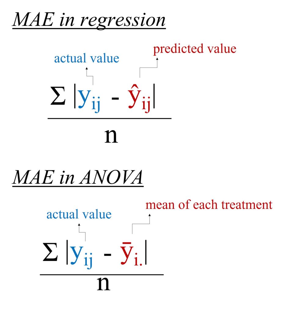
Mean Absolute Error (MAE) is a metric used to measure the accuracy of a model’s predictions. It calculates the average magnitude of the errors in a set of predictions, without considering their direction. In other words, MAE measures the average absolute difference between the actual values and the predicted values. MAE is typically used in the context of regression analysis and prediction error evaluation, rather than in ANOVA (Analysis of Variance), which focuses on comparing the means of different groups. However, the concept of measuring error can still be relevant when assessing the fit of a model in ANOVA contexts.

Today, I’ll explain how to calculate MAE when conducting ANOVA.

Here is one dataset. Let’s say this data represents yield in response to different fertilizer types.

Fertilizer	Yield
Control	12.2
Control	12.4
Control	11.9
Control	11.3
Control	11.8
Control	12.1
Control	13.1
Control	12.7
Control	12.4
Control	11.4
Slow	16.6
Slow	15.8
Slow	16.5
Slow	15.0
Slow	15.4
Slow	15.6
Slow	15.8
Slow	15.8
Slow	16.0
Slow	15.8
Fast	9.5
Fast	9.5
Fast	9.6
Fast	8.8
Fast	9.5
Fast	9.8
Fast	9.1
Fast	10.3
Fast	9.5
Fast	8.5

Fertilizer is an experimental factor, and yield is the final outcome from that factor. Therefore, fertilizer is the independent variable (x), while yield is the dependent variable (y). Each yield value is indicated as y_ij where i is fertilizers and j is replicates. It means y₁₁ will be the first replicate at control, which is 12.2

x	y_ij
Fertilizer	Yield
Control	12.2
Control	12.4
Control	11.9
Control	11.3
Control	11.8
Control	12.1
Control	13.1
Control	12.7
Control	12.4
Control	11.4
Slow	16.6
Slow	15.8
Slow	16.5
Slow	15.0
Slow	15.4
Slow	15.6
Slow	15.8
Slow	15.8
Slow	16.0
Slow	15.8
Fast	9.5
Fast	9.5
Fast	9.6
Fast	8.8
Fast	9.5
Fast	9.8
Fast	9.1
Fast	10.3
Fast	9.5
Fast	8.5

Next, I’ll calculate the grain mean (ȳ_..) across all fertilizers.

x	y_ij	ȳ..
Fertilizer	Yield	Grand mean
Control	12.2	12.46
Control	12.4	12.46
Control	11.9	12.46
Control	11.3	12.46
Control	11.8	12.46
Control	12.1	12.46
Control	13.1	12.46
Control	12.7	12.46
Control	12.4	12.46
Control	11.4	12.46
Slow	16.6	12.46
Slow	15.8	12.46
Slow	16.5	12.46
Slow	15.0	12.46
Slow	15.4	12.46
Slow	15.6	12.46
Slow	15.8	12.46
Slow	15.8	12.46
Slow	16.0	12.46
Slow	15.8	12.46
Fast	9.5	12.46
Fast	9.5	12.46
Fast	9.6	12.46
Fast	8.8	12.46
Fast	9.5	12.46
Fast	9.8	12.46
Fast	9.1	12.46
Fast	10.3	12.46
Fast	9.5	12.46
Fast	8.5	12.46

Next, I’ll calculate the mean of each fertilizer, and it will be written as ȳ_i.

x	y_ij	ȳ..	ȳ_i.
Fertilizer	Yield	Grand mean	Fertilizer mean
Control	12.2	12.46	12.13
Control	12.4	12.46	12.13
Control	11.9	12.46	12.13
Control	11.3	12.46	12.13
Control	11.8	12.46	12.13
Control	12.1	12.46	12.13
Control	13.1	12.46	12.13
Control	12.7	12.46	12.13
Control	12.4	12.46	12.13
Control	11.4	12.46	12.13
Slow	16.6	12.46	15.83
Slow	15.8	12.46	15.83
Slow	16.5	12.46	15.83
Slow	15.0	12.46	15.83
Slow	15.4	12.46	15.83
Slow	15.6	12.46	15.83
Slow	15.8	12.46	15.83
Slow	15.8	12.46	15.83
Slow	16.0	12.46	15.83
Slow	15.8	12.46	15.83
Fast	9.5	12.46	9.4
Fast	9.5	12.46	9.4
Fast	9.6	12.46	9.4
Fast	8.8	12.46	9.4
Fast	9.5	12.46	9.4
Fast	9.8	12.46	9.4
Fast	9.1	12.46	9.4
Fast	10.3	12.46	9.4
Fast	9.5	12.46	9.4
Fast	8.5	12.46	9.4

Then, I will subtract the grand mean (ȳ..) from the fertilizer mean (ȳ_i_.), and this is called the fertilizer effect (or treatment effect).

x	y_ij	ȳ..	ȳ_i.	ȳi. – ȳ..
Fertilizer	Yield	Grand mean	Fertilizer mean	Fertilizer effect
Control	12.2	12.46	12.13	-0.33 (=12.13 – 12.46)
Control	12.4	12.46	12.13	-0.33
Control	11.9	12.46	12.13	-0.33
Control	11.3	12.46	12.13	-0.33
Control	11.8	12.46	12.13	-0.33
Control	12.1	12.46	12.13	-0.33
Control	13.1	12.46	12.13	-0.33
Control	12.7	12.46	12.13	-0.33
Control	12.4	12.46	12.13	-0.33
Control	11.4	12.46	12.13	-0.33
Slow	16.6	12.46	15.83	3.37
Slow	15.8	12.46	15.83	3.37
Slow	16.5	12.46	15.83	3.37
Slow	15.0	12.46	15.83	3.37
Slow	15.4	12.46	15.83	3.37
Slow	15.6	12.46	15.83	3.37
Slow	15.8	12.46	15.83	3.37
Slow	15.8	12.46	15.83	3.37
Slow	16.0	12.46	15.83	3.37
Slow	15.8	12.46	15.83	3.37
Fast	9.5	12.46	9.4	-3.05
Fast	9.5	12.46	9.4	-3.05
Fast	9.6	12.46	9.4	-3.05
Fast	8.8	12.46	9.4	-3.05
Fast	9.5	12.46	9.4	-3.05
Fast	9.8	12.46	9.4	-3.05
Fast	9.1	12.46	9.4	-3.05
Fast	10.3	12.46	9.4	-3.05
Fast	9.5	12.46	9.4	-3.05
Fast	8.5	12.46	9.4	-3.05

Next, I will subtract the fertilizer mean (ȳ_i_.) from each yield value (y_ij), and this is called residuals (or errors).

x	y_ij	ȳ..	ȳ_i.	ȳi. – ȳ..	y_ij – ȳ_i.
Fertilizer	Yield	Grand mean	Fertilizer mean	Fertilizer effect	Residuals
Control	12.2	12.46	12.13	-0.33	0.07 (=12.2 – 12.13)
Control	12.4	12.46	12.13	-0.33	0.27
Control	11.9	12.46	12.13	-0.33	-0.23
Control	11.3	12.46	12.13	-0.33	-0.83
Control	11.8	12.46	12.13	-0.33	-0.33
Control	12.1	12.46	12.13	-0.33	-0.03
Control	13.1	12.46	12.13	-0.33	0.97
Control	12.7	12.46	12.13	-0.33	0.57
Control	12.4	12.46	12.13	-0.33	0.27
Control	11.4	12.46	12.13	-0.33	-0.73
Slow	16.6	12.46	15.83	3.37	0.77
Slow	15.8	12.46	15.83	3.37	-0.03
Slow	16.5	12.46	15.83	3.37	0.67
Slow	15.0	12.46	15.83	3.37	-0.83
Slow	15.4	12.46	15.83	3.37	-0.43
Slow	15.6	12.46	15.83	3.37	-0.23
Slow	15.8	12.46	15.83	3.37	-0.03
Slow	15.8	12.46	15.83	3.37	-0.03
Slow	16.0	12.46	15.83	3.37	0.17
Slow	15.8	12.46	15.83	3.37	-0.03
Fast	9.5	12.46	9.4	-3.05	0.09
Fast	9.5	12.46	9.4	-3.05	0.09
Fast	9.6	12.46	9.4	-3.05	0.19
Fast	8.8	12.46	9.4	-3.05	-0.61
Fast	9.5	12.46	9.4	-3.05	0.09
Fast	9.8	12.46	9.4	-3.05	0.39
Fast	9.1	12.46	9.4	-3.05	-0.31
Fast	10.3	12.46	9.4	-3.05	0.89
Fast	9.5	12.46	9.4	-3.05	0.09
Fast	8.5	12.46	9.4	-3.05	-0.91

Finally, I’ll calculate the total variation. I will subtract the grand mean (ȳ..) from each yield value (y_ij), and this is called Total.

x	y_ij	ȳ..	ȳ_i.	ȳi. – ȳ..	y_ij – ȳ_i.	y_ij – ȳ_..
Fertilizer	Yield	Grand mean	Fertilizer mean	Fertilizer effect	Residuals	Total
Control	12.2	12.46	12.13	-0.33	0.07	-0.26
Control	12.4	12.46	12.13	-0.33	0.27	-0.06
Control	11.9	12.46	12.13	-0.33	-0.23	-0.56
Control	11.3	12.46	12.13	-0.33	-0.83	-1.16
Control	11.8	12.46	12.13	-0.33	-0.33	-0.66
Control	12.1	12.46	12.13	-0.33	-0.03	-0.36
Control	13.1	12.46	12.13	-0.33	0.97	0.64
Control	12.7	12.46	12.13	-0.33	0.57	0.24
Control	12.4	12.46	12.13	-0.33	0.27	-0.06
Control	11.4	12.46	12.13	-0.33	-0.73	-1.06
Slow	16.6	12.46	15.83	3.37	0.77	4.14
Slow	15.8	12.46	15.83	3.37	-0.03	3.34
Slow	16.5	12.46	15.83	3.37	0.67	4.04
Slow	15.0	12.46	15.83	3.37	-0.83	2.54
Slow	15.4	12.46	15.83	3.37	-0.43	2.94
Slow	15.6	12.46	15.83	3.37	-0.23	3.14
Slow	15.8	12.46	15.83	3.37	-0.03	3.34
Slow	15.8	12.46	15.83	3.37	-0.03	3.34
Slow	16.0	12.46	15.83	3.37	0.17	3.54
Slow	15.8	12.46	15.83	3.37	-0.03	3.34
Fast	9.5	12.46	9.4	-3.05	0.09	-2.96
Fast	9.5	12.46	9.4	-3.05	0.09	-2.96
Fast	9.6	12.46	9.4	-3.05	0.19	-2.86
Fast	8.8	12.46	9.4	-3.05	-0.61	-3.66
Fast	9.5	12.46	9.4	-3.05	0.09	-2.96
Fast	9.8	12.46	9.4	-3.05	0.39	-2.66
Fast	9.1	12.46	9.4	-3.05	-0.31	-3.36
Fast	10.3	12.46	9.4	-3.05	0.89	-2.16
Fast	9.5	12.46	9.4	-3.05	0.09	-2.96
Fast	8.5	12.46	9.4	-3.05	-0.91	-3.96

I calculated each variation, and we can prove Total variation = Treatment effect + Error.

Total Variation refers to the overall variability in the data.
Treatment Effect captures the variability attributable to the differences between treatment groups or conditions.
Error (or residual variation) accounts for the variability within each treatment group that is not explained by the treatment itself.

For example, in the first yield value in the table, -0.26 = – 0.33 + 0.07

Also, yield can be partitioned into yield= grand mean + Treatment effect + Error.

For example, in the first yield value in the table, 12.2 = 12.46 – 0.33 + 0.07

and it could be written as y_ij = μ + τ_i+ ε_ij where μ is the grand mean, τi is the treatment effect, and εij is residuals.

From now on, I’m interested in the magnitude of each variation. When summing them, you’ll find that the total is always 0. The sum of the deviations (each value – the mean) is always 0. To avoid this result, I’ll square each deviation.

x	y_ij	ȳ..	ȳ_i.	ȳi. – ȳ..	y_ij – ȳ_i.	y_ij – ȳ_..	(ȳ_i. – ȳ_..)²	(y_ij – ȳ_i.)²	(y_ij – ȳ_..)²
Fertilizer	Yield	Grand mean	Fertilizer mean	Fertilizer effect	Residuals	Total	Fertilizer effect^2	Residuals^2	Total^2
Control	12.2	12.46	12.13	-0.33	0.07	-0.26	0.11	0.00	0.07
Control	12.4	12.46	12.13	-0.33	0.27	-0.06	0.11	0.07	0.00
Control	11.9	12.46	12.13	-0.33	-0.23	-0.56	0.11	0.05	0.31
Control	11.3	12.46	12.13	-0.33	-0.83	-1.16	0.11	0.69	1.34
Control	11.8	12.46	12.13	-0.33	-0.33	-0.66	0.11	0.11	0.43
Control	12.1	12.46	12.13	-0.33	-0.03	-0.36	0.11	0.00	0.13
Control	13.1	12.46	12.13	-0.33	0.97	0.64	0.11	0.94	0.41
Control	12.7	12.46	12.13	-0.33	0.57	0.24	0.11	0.32	0.06
Control	12.4	12.46	12.13	-0.33	0.27	-0.06	0.11	0.07	0.00
Control	11.4	12.46	12.13	-0.33	-0.73	-1.06	0.11	0.53	1.12
Slow	16.6	12.46	15.83	3.37	0.77	4.14	11.38	0.59	17.17
Slow	15.8	12.46	15.83	3.37	-0.03	3.34	11.38	0.00	11.18
Slow	16.5	12.46	15.83	3.37	0.67	4.04	11.38	0.45	16.35
Slow	15.0	12.46	15.83	3.37	-0.83	2.54	11.38	0.69	6.47
Slow	15.4	12.46	15.83	3.37	-0.43	2.94	11.38	0.18	8.66
Slow	15.6	12.46	15.83	3.37	-0.23	3.14	11.38	0.05	9.88
Slow	15.8	12.46	15.83	3.37	-0.03	3.34	11.38	0.00	11.18
Slow	15.8	12.46	15.83	3.37	-0.03	3.34	11.38	0.00	11.18
Slow	16.0	12.46	15.83	3.37	0.17	3.54	11.38	0.03	12.56
Slow	15.8	12.46	15.83	3.37	-0.03	3.34	11.38	0.00	11.18
Fast	9.5	12.46	9.4	-3.05	0.09	-2.96	9.28	0.01	8.74
Fast	9.5	12.46	9.4	-3.05	0.09	-2.96	9.28	0.01	8.74
Fast	9.6	12.46	9.4	-3.05	0.19	-2.86	9.28	0.04	8.16
Fast	8.8	12.46	9.4	-3.05	-0.61	-3.66	9.28	0.37	13.37
Fast	9.5	12.46	9.4	-3.05	0.09	-2.96	9.28	0.01	8.74
Fast	9.8	12.46	9.4	-3.05	0.39	-2.66	9.28	0.15	7.06
Fast	9.1	12.46	9.4	-3.05	-0.31	-3.36	9.28	0.10	11.27
Fast	10.3	12.46	9.4	-3.05	0.89	-2.16	9.28	0.79	4.65
Fast	9.5	12.46	9.4	-3.05	0.09	-2.96	9.28	0.01	8.74
Fast	8.5	12.46	9.4	-3.05	-0.91	-3.96	9.28	0.83	15.66
						Σ	207.68	7.11	214.79

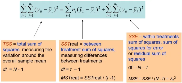
From now on, we can sum each squared variation. Therefore, I will refer to them as the sum of squared Treatment (Fertilizer), the Sum of Squared Errors (residuals), and the Sum of Squared Total. As abbreviations, I’ll write them as SS_Treatment , SS_Error, and SS_Total and we can also prove the below formula.

SS_Total = SS_Treatment + SS_Error

which is 214.79 = 207.68 + 7.11

and mathematical formula, it can be written as

Σ(y_ij - ȳ_..)² = Σ(ȳ_i. - ȳ_..)² + Σ(y_ij - ȳ_i.)²

As summarized in the figure below.

■ What is Mean Squared Error (MSE)?

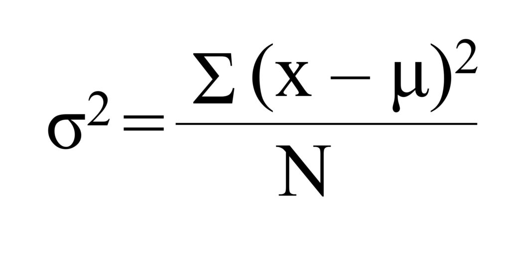
Do you know the equation of variance?

If we know the population mean, we can calculate population variance (σ²) as follows.

However, in most cases, we do not know the population mean, and therefore, we take some samples (n) from the population and will use the mean of samples to calculate sample variance as follows.

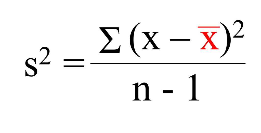
Let’s connect the concept of the variance equation above with the concepts of SS_Treatment , SS_Error, and SS_Total

Variance is calculated as the Sum of Squared (SS) divided by the degree of freedom (n-1).

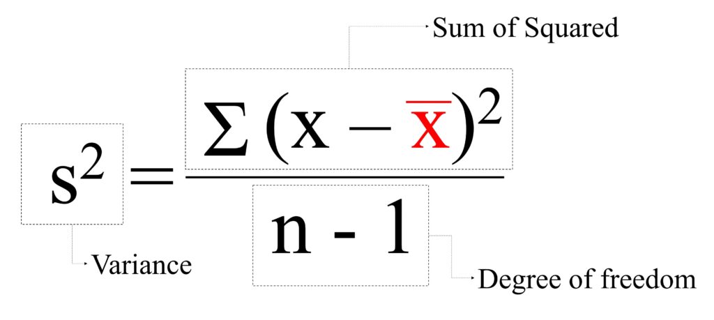
We already calculated SS_Treatment , SS_Error, and SS_Total and degree of freedom of each case is calculated as

df SS_Total = N - 1 (where N is total number of samples)
df SS_Treatment = t - 1 (where t is number of levels of the treatment)
df SS_Error = N- t

So, we can calculate the variance of Total, Treatment, and Error as follows.

▪ Variance of Total = 214.79 / 30 = 7.1597
▪ Variance of Treatment = 207.69 / (3 – 1) = 103.845
▪ Variance of Error = 7.11 / (30 – 3) = 0.263

Also, we can refer to them as the Mean Squared of Total, Treatment, and Error since we divide the Sum of Squares by the sample size (specifically n-1 for sampling data). Therefore, the Mean Squared Treatment, and the Mean Squared Error are equivalent to the Variance of Treatment and Error, respectively. In statistics, the Mean Squared Error is often referred to as MSE for simplicity.

Therefore, in the dataset, the MSE is 0.236, which represents the variance of the error in the data.

Let’s check this calculation is correct using a statistical program. I use R.

First, I’ll upload the dataset.

if(!require(readr)) install.packages("readr")
library(readr)
github="https://raw.githubusercontent.com/agronomy4future/raw_data_practice/refs/heads/main/Fertilizer%20(One%20Way%20ANOVA).csv"
df= data.frame(read_csv(url(github), show_col_types=FALSE))

head(df,5)
  Fertilizer Yield Height
1    Control  12.2     45
2    Control  12.4     52
3    Control  11.9     42
4    Control  11.3     35
5    Control  11.8     40
.
.
.

I will conduct a statistical analysis using One-Way ANOVA.

model= aov(Yield ~ Fertilizer, data=df)
summary (model)

            Df Sum Sq Mean Sq F value Pr(>F)    
Fertilizer   2 207.68  103.84   394.3 <2e-16 ***
Residuals   27   7.11    0.26

MSE is the same as what I calculate manually.

■ How about Mean Absolute Error (MAE)?

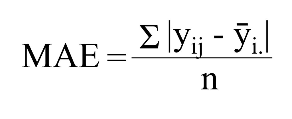
This is the equation for MAE. It’s simple: instead of squaring the residuals, you take the absolute value and divide by the number of samples (n).

This is the difference between MSE and MAE.

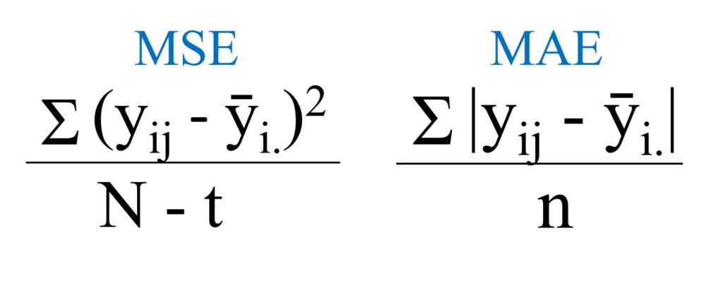
Let’s calculate MAE according to the equation.

x	y_ij	ȳ..	ȳ_i.	ȳi. – ȳ..	y_ij – ȳ_i.	y_ij – ȳ_..	(ȳ_i. – ȳ_..)²	(y_ij – ȳ_i.)²	(y_ij – ȳ_..)²	\|y_ij – ȳ_i.\|
Fertilizer	Yield	Grand mean	Fertilizer mean	Fertilizer effect	Residuals	Total	Fertilizer effect^2	Residuals^2	Total^2	Absolute Error
Control	12.2	12.46	12.13	-0.33	0.07	-0.26	0.11	0.00	0.07	0.07
Control	12.4	12.46	12.13	-0.33	0.27	-0.06	0.11	0.07	0.00	0.27
Control	11.9	12.46	12.13	-0.33	-0.23	-0.56	0.11	0.05	0.31	0.23
Control	11.3	12.46	12.13	-0.33	-0.83	-1.16	0.11	0.69	1.34	0.83
Control	11.8	12.46	12.13	-0.33	-0.33	-0.66	0.11	0.11	0.43	0.33
Control	12.1	12.46	12.13	-0.33	-0.03	-0.36	0.11	0.00	0.13	0.03
Control	13.1	12.46	12.13	-0.33	0.97	0.64	0.11	0.94	0.41	0.97
Control	12.7	12.46	12.13	-0.33	0.57	0.24	0.11	0.32	0.06	0.57
Control	12.4	12.46	12.13	-0.33	0.27	-0.06	0.11	0.07	0.00	0.27
Control	11.4	12.46	12.13	-0.33	-0.73	-1.06	0.11	0.53	1.12	0.73
Slow	16.6	12.46	15.83	3.37	0.77	4.14	11.38	0.59	17.17	0.77
Slow	15.8	12.46	15.83	3.37	-0.03	3.34	11.38	0.00	11.18	0.03
Slow	16.5	12.46	15.83	3.37	0.67	4.04	11.38	0.45	16.35	0.67
Slow	15.0	12.46	15.83	3.37	-0.83	2.54	11.38	0.69	6.47	0.83
Slow	15.4	12.46	15.83	3.37	-0.43	2.94	11.38	0.18	8.66	0.43
Slow	15.6	12.46	15.83	3.37	-0.23	3.14	11.38	0.05	9.88	0.23
Slow	15.8	12.46	15.83	3.37	-0.03	3.34	11.38	0.00	11.18	0.03
Slow	15.8	12.46	15.83	3.37	-0.03	3.34	11.38	0.00	11.18	0.03
Slow	16.0	12.46	15.83	3.37	0.17	3.54	11.38	0.03	12.56	0.17
Slow	15.8	12.46	15.83	3.37	-0.03	3.34	11.38	0.00	11.18	0.03
Fast	9.5	12.46	9.4	-3.05	0.09	-2.96	9.28	0.01	8.74	0.09
Fast	9.5	12.46	9.4	-3.05	0.09	-2.96	9.28	0.01	8.74	0.09
Fast	9.6	12.46	9.4	-3.05	0.19	-2.86	9.28	0.04	8.16	0.19
Fast	8.8	12.46	9.4	-3.05	-0.61	-3.66	9.28	0.37	13.37	0.61
Fast	9.5	12.46	9.4	-3.05	0.09	-2.96	9.28	0.01	8.74	0.09
Fast	9.8	12.46	9.4	-3.05	0.39	-2.66	9.28	0.15	7.06	0.39
Fast	9.1	12.46	9.4	-3.05	-0.31	-3.36	9.28	0.10	11.27	0.31
Fast	10.3	12.46	9.4	-3.05	0.89	-2.16	9.28	0.79	4.65	0.89
Fast	9.5	12.46	9.4	-3.05	0.09	-2.96	9.28	0.01	8.74	0.09
Fast	8.5	12.46	9.4	-3.05	-0.91	-3.96	9.28	0.83	15.66	0.91
						Σ	207.68	7.11	214.79	11.18

MAE = 11.18 / 30 = 0.373

Mean Absolute Error (MAE) is calculated as 0.373. Let’s check this calculation is correct.

if(!require(Metrics)) install.packages("Metrics")
library(Metrics)

model= aov(Yield ~ Fertilizer, data=df)

mae(df$Yield, predict(model))
0.3726667

The value is the same.

Agronomy4future

Stories about cereals and statistics (plus coding). We aim to develop open-source code for agronomy.

Understanding Mean Absolute Error (MAE) in ANOVA: A Step-by-Step Guide to Calculation in Excel

October 27, 2024 JK

■ What is Mean Squared Error (MSE)?

■ How about Mean Absolute Error (MAE)?