[STAT Article] Steps to Calculate Log-Likelihood Prior to AIC and BIC: [Part 1] regression model

Here I have one dataset.
df= data.frame(
  Length= c(5.3, 6.14, 6.56, 6.26, 6.24, 5.65, 6.02, 6.59, 5.89, 6.1),
  Width= c(2.06, 3.73, 3.33, 3.13, 3.5, 3.16, 3.82, 3.11, 2.87, 3.58),
  Area= c(8.04, 17.51, 17.06, 15.54, 17.13, 13.76, 17.43, 16, 12.51, 15.84),
  Weight= c(15.73, 44.02, 42.53, 37.59, 42.76, 32, 43.76, 39.06, 28.22, 38.55)
)

print(df)
   Length Width  Area Weight
1    5.30  2.06  8.04  15.73
2    6.14  3.73 17.51  44.02
3    6.56  3.33 17.06  42.53
4    6.26  3.13 15.54  37.59
5    6.24  3.50 17.13  42.76
6    5.65  3.16 13.76  32.00
7    6.02  3.82 17.43  43.76
8    6.59  3.11 16.00  39.06
9    5.89  2.87 12.51  28.22
10   6.10  3.58 15.84  38.55
I want to predict grain weight using grain dimension data such as length, width, and area, and identify the best prediction model for estimating grain weight. As a result, I developed the following models.
model_1=lm (Weight ~ Area + Length + Width, data=df)
model_2=lm (Weight ~ Area + Length, data=df)
model_3=lm (Weight ~ Area + Width, data=df)
model_4=lm (Weight ~ Length + Width, data=df)
model_5=lm (Weight ~ Length, data=df)
model_6=lm (Weight ~ Width, data=df)
model_7=lm (Weight ~ Area, data=df)
and I’ll calculate Log-likelihood for each model. To do that, I need to know each model equation.
models= list(
  lm(Weight ~ Area + Length + Width, data = df),
  lm(Weight ~ Area + Length, data = df),
  lm(Weight ~ Area + Width, data = df),
  lm(Weight ~ Length + Width, data = df),
  lm(Weight ~ Length, data = df),
  lm(Weight ~ Width, data = df),
  lm(Weight ~ Area, data = df)
)

print_equation= function(model, model_number) {
  dependent_var= as.character(formula(model)[[2]])
  coeffs= coef(model)
  intercept= round(coeffs[1], 4)
  terms= names(coeffs)[-1]
  term_equations= paste(paste0(round(coeffs[-1], 4), "*", terms), collapse= " + ")
  equation= paste0("Model ", model_number, ": ", dependent_var, " = ", intercept, " + ", term_equations)
  cat(equation, "\n")
}

for (i in 1:length(models)) {
  print_equation(models[[i]], i)
}

###
Model 1: Weight = -2.9824 + 3.3395*Area + -1.0947*Length + -1.3356*Width
Model 2: Weight = -7.9964 + 3.0313*Area + -0.214*Length
Model 3: Weight = -8.8793 + 3.0234*Area + -0.0923*Width
Model 4: Weight = -58.1413 + 8.9366*Length + 12.4725*Width
Model 5: Weight = -73.9139 + 18.1623*Length
Model 6: Weight = -16.5345 + 16.4003*Width
Model 7: Weight = -8.9535 + 3.0086*Area
Now, I obtained each model equation, and I’ll calculate Log-likelihood
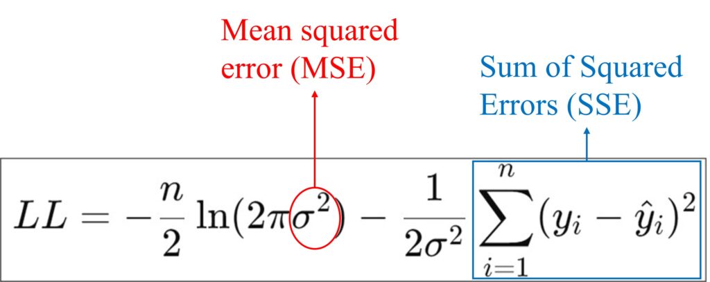
For a linear regression model, the Log-Likelihood (LL) is defined as:

where:
n is the number of observations
𝑦𝑖 is the observed value for independent variable (here, it's Weight)
ŷi is the predicted value of Weight based on the model
σ2 is the variance of residuals (errors); in other words, it is also called the Mean Squared Error (MSE)
I’ll calculate Log-likelihood for the model 7
| Area | Weight (𝑦𝑖) | Prediction (ŷi) | Errors (𝑦𝑖 – ŷi) | Squared Errors (𝑦𝑖 – ŷi)2 |
| 8.04 | 15.73 | 15.24 | 0.49 | 0.24 |
| 17.51 | 44.02 | 43.73 | 0.29 | 0.09 |
| 17.06 | 42.53 | 42.37 | 0.16 | 0.02 |
| 15.54 | 37.59 | 37.80 | -0.21 | 0.04 |
| 17.13 | 42.76 | 42.58 | 0.18 | 0.03 |
| 13.76 | 32.00 | 32.44 | -0.44 | 0.20 |
| 17.43 | 43.76 | 43.49 | 0.27 | 0.07 |
| 16.00 | 39.06 | 39.18 | -0.12 | 0.02 |
| 12.51 | 28.22 | 28.68 | -0.46 | 0.22 |
| 15.84 | 38.55 | 38.70 | -0.15 | 0.02 |
| Sum of Squared Errors (SSE) ∑ (𝑦𝑖 – ŷi)2 = 0.957 |
For example, in the Prediction column, 15.24 was calculated based on the equation: Weight = -8.9535 + 3.0086*Area, which is -8.9535 + 3.0086*8.04 = 15.24, and the difference (𝑦𝑖 – ŷi) between actual and predicted value will be error, which is 15.73 - 15.24 = 0.49
σ2 is the variance of errors, and it will be calculated ∑(𝑦𝑖 - ŷi)2 / n. Usually, MSE is calculated as ∑(𝑦𝑖 - ŷi)2 / (n - p), but in the likelihood function, it is calculated as SSE/n, which is ∑ (𝑦𝑖 - ŷi)2 / n
Mean squared error (MSE)
0.957 / 10 = 0.0957

Now we can calculate Log-Likelihood for the model 7.
LL= -10/2*ln(2*3.14*0.0957) - 0.957/(2*0.0957) ≈ -2.45
The Log-Likelihood for the model 7 is around -2.45
let’s verify this value is correct using R.
logLik(model_7)

'log Lik.' -2.455688 (df=3)
We can verify the calculation for Log-Likelihood is correct. df=3 correspond to 2 model parameters (intercept and slope), with 1 additional degree of freedom associated with the residual variance.
Now, let’s understand how to calculate the Log-Likelihood manually. We’ll calculate it step by step in R, not simply using logLik(model_7).
residuals= resid(model_7)
SSE=sum(residuals^2)
MSE= SSE / length(df$Weight)

LL= -length(df$Weight)/2*log(2*pi*MSE) - SSE/(2*MSE)

cat("Log-likelihood:", LL, "\n")
Log-likelihood: -2.455688
Then, now we can calculate Akaike information criterion (AIC) and Bayesian Information Criterion (BIC).
The Akaike Information Criterion (AIC) is a statistical measure used to compare and evaluate different models based on their goodness of fit and complexity. It helps to identify the model that best balances fit (how well the model explains the data) and complexity (how many parameters the model uses).
The formula for AIC:
AIC= 2*k - 2*ln(L)

where:
k is the number of parameters in the model
ln(L) is the likelihood of the model
We already calculated Log-Likelihood, and k is 3 (intercept, slope and error) in the model. Also, given this, the number of parameters, k used in the AIC formula is 3 (2 coefficients + residual variance).
Therefore, AIC is calculated as 2*3 - 2*-2.455688 = 10.91138
let’s verify this value is correct using R.
AIC (model_7)
10.91138
My calculation is correct!!
Let’s calculate BIC. The Bayesian Information Criterion (BIC) is another model selection criterion, similar to the Akaike Information Criterion (AIC), but it applies a stronger penalty for models with more parameters. The goal of BIC, like AIC, is to balance model fit (how well the model explains the data) with model complexity (how many parameters the model uses).
The formula for BIC:
BIC= k*ln(n) - 2*ln(L)

where:
k is the number of parameters in the model
ln(L) is the likelihood of the model
n is the number of data points.
Again, we already calculated Log-Likelihood, and k is 3 (intercept, slope and error) in the model. Also, given this, the number of parameters, k used in the BIC formula is 3 (2 coefficients + residual variance).
Therefore, AIC is calculated as 3*log(10) - (2*-2.455688) = 11.81913
let’s verify this value is correct using R.
BIC (model_7)
11.81913
Let’s summary all.
| Model | Model structure | Log-Likelihood | AIC | BIC |
| model_1 | Weight ~ Area + Length + Width | -1.60 | 13.2 | 14.7 |
| model_2 | Weight ~ Area + Length | -2.34 | 12.7 | 13.9 |
| model_3 | Weight ~ Area + Width | -2.4 | 12.9 | 14.1 |
| model_4 | Weight ~ Length + Width | -16.3 | 40.6 | 41.8 |
| model_5 | Weight ~ Length | -30.5 | 67.0 | 67.9 |
| model_6 | Weight ~ Width | -25.2 | 56.3 | 57.2 |
| model_7 | Weight ~ Area | -2.5 | 11.0 | 11.8 |
In both AIC (Akaike Information Criterion) and BIC (Bayesian Information Criterion), a lower value is better. These criteria are used to evaluate and compare different statistical models, balancing model fit and complexity. AIC is used to select the model that best explains the data with a penalty for the number of parameters (complexity). A lower AIC value indicates a better model, as it suggests the model provides a good fit with fewer parameters, thus avoiding overfitting. BIC is similar to AIC, but with a stronger penalty for the number of parameters, especially when the sample size is large. A lower BIC also indicates a better model.
So, in this case, model_7 would be better model.
■ Practice
Let’s practice calculating Log-Likelihood, AIC and BIC with another dataset.
if(!require(readr)) install.packages("readr")
library(readr)
github="https://raw.githubusercontent.com/agronomy4future/raw_data_practice/refs/heads/main/ML_Practice_Grain_Dimension.csv"
df= data.frame(read_csv(url(github), show_col_types=FALSE))

head(df,5)
  Genotype Length_mm Width_mm Area_mm_2 GW_mg
1      cv1      4.86     2.12      7.56 14.44
2      cv1      5.01     1.94      7.25 13.67
3      cv1      5.54     1.97      7.99 15.55
4      cv1      3.84     1.99      5.86 10.32
5      cv1      5.30     2.06      8.04 15.66
.
.
.
This is a huge dataset containing 95950 data rows. Using this dataset, I want to find the best model to predict grain weight (GW_mg).
1) Create models you want to compare
2) Calculate Log-Likelihood, but not using logLik()
3) Calculate AIC and BIC, but not using AIC() and BIC()
