---

SAS Studio is a web version of the SAS program, and it can be used for free. As my current license for the statistical program I’ve been using is about to expire, I was searching for alternatives. Upon discovering SAS Studio, I decided to give it a try. Although I have never used SAS before, I’ve decided to take this opportunity to learn. I will now summarize the very basic learning materials I have covered up to this point.

First, go to the webpage mentioned above and access SAS Studio. To access it, you’ll need a SAS account. Creating an account is easy on the SAS website.

Now, when you click on Access Now, you will be redirected to the SAS® OnDemand for Academics Dashboard.”

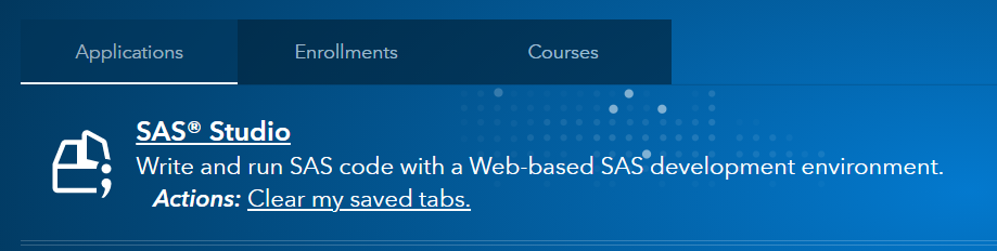
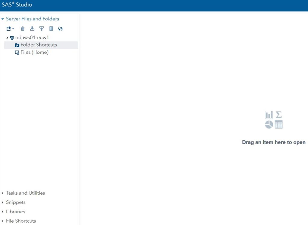
To access SAS Studio, click on ‘SAS® Studio.’ The basic SAS Studio window will appear. Now, let’s proceed to explore various functionalities within this interface.

---

---

1. to upload data

First, let’s create a folder. In the ‘Files (Home)’ section, right-click and then choose New > Folder

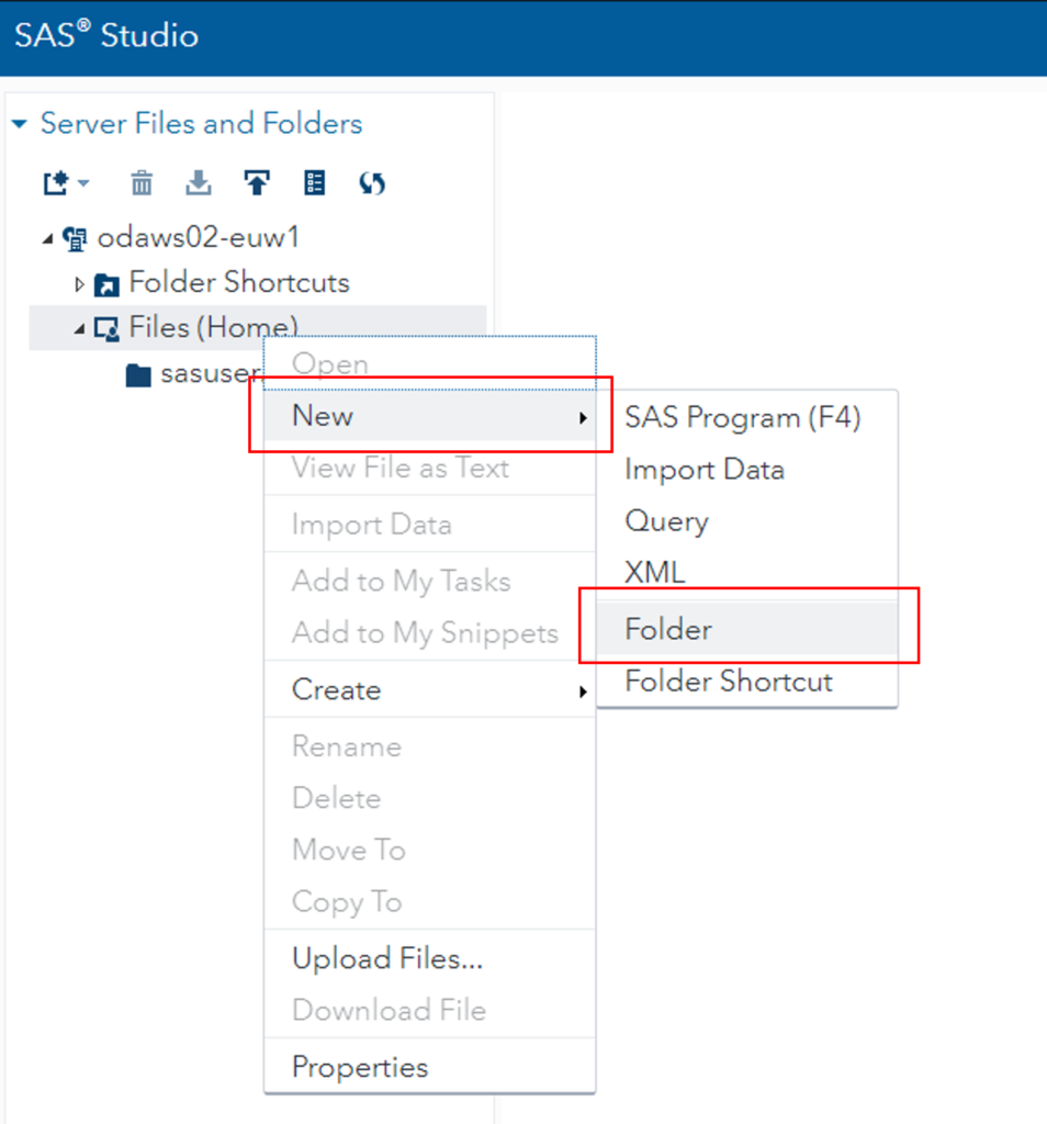
A window for creating a new folder will appear. I will name the folder ‘SAS Programming.’ Now, click on the newly created ‘SAS Programming’ folder and then click the upload button. You can also right-click on the folder and choose Upload Files.

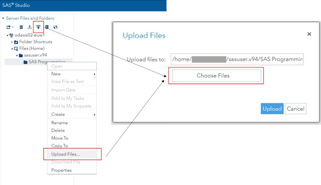
Click on Choose Files and select the file you want to upload. In my case, I have uploaded a file named ‘DataA.xlsx.’ Once uploaded, clicking on ‘DataA.xlsx’ will open a code window below. One of the advantages of SAS Studio is that it displays the code corresponding to your actions, providing a natural way to learn SAS programming. Now, click the ‘Run’ button above. The shortcut for this is F3.”

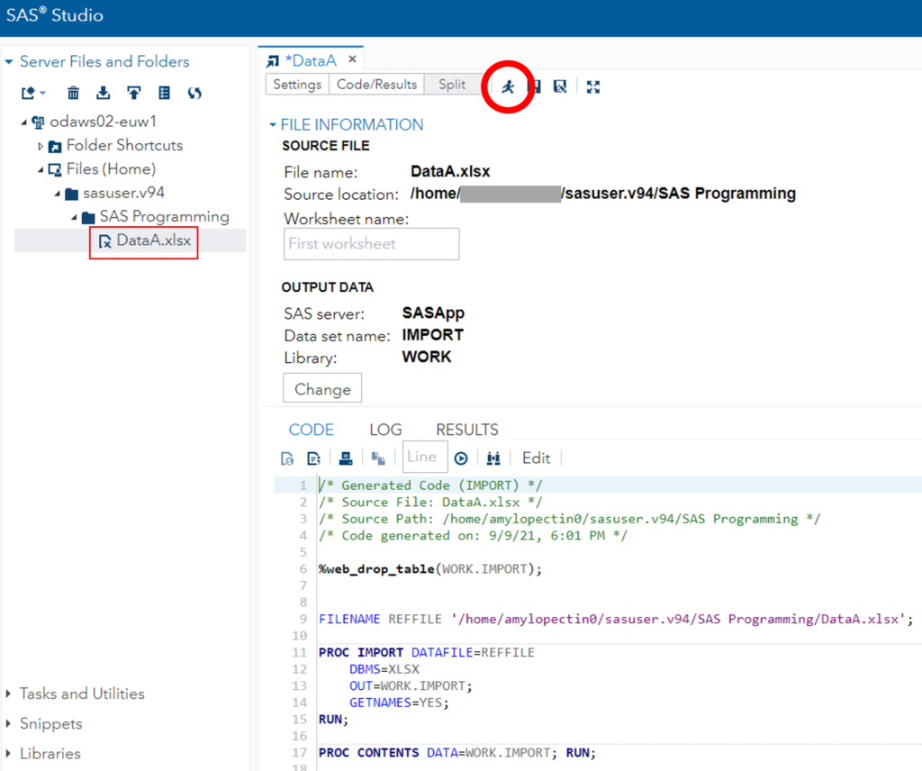
Upon doing so, you will see the OUTPUT DATA tab, where you can inspect the uploaded data.

---

---

2. to convert the uploaded data into a library table

To perform statistical analysis in SAS Studio, you need to transform this data into a data table within the SAS Studio Library. First, let’s create a new library.

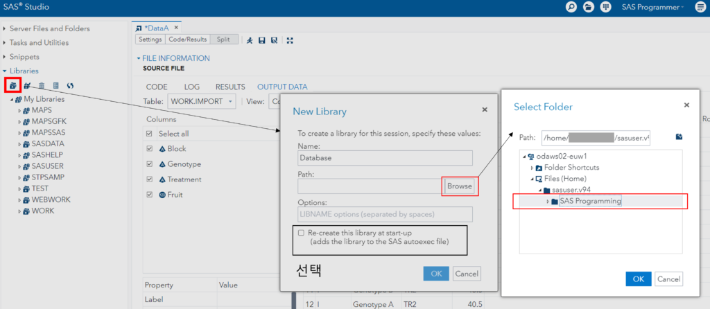
From the left menu, select ‘Library,’ then click the ‘New Library’ icon. You can click My Libraries and right-click to create a new library as well. For my case, I’ll name the new library ‘Database’ and click ‘Browse’ to select the newly created folder ‘SAS Programming’ as the location. Also, select Re-create this library at start-up.

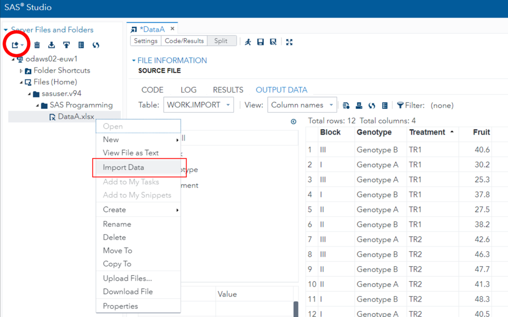
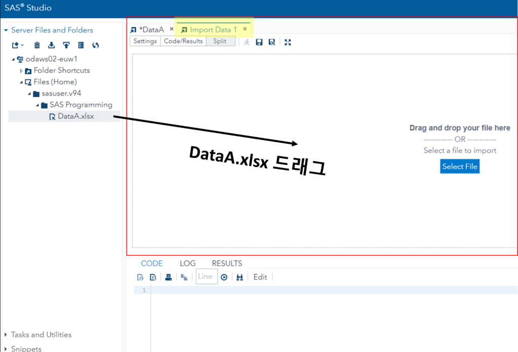
Now, the new library named ‘Database’ has been created. Let’s go back to the Server Files and Folders menu. Click on the ‘Import Data’ icon at the top left, or right-click on the uploaded data ‘DataA.xlsx’ and select Import Data.

“Upon doing so, a new tab named ‘Import Data 1’ will appear. Here, click and drag the uploaded ‘DataA.xlsx’ from the left menu into the window, or click Select File to choose ‘DataA’.”

Upon doing so, a window like the one below will appear. In the OUTPUT DATA section, set the path of the Library to the ‘DATABASE’ we created earlier, and for the Library Data Table, specify the name ‘Yield.’ Then, click the ‘Run’ button again.”

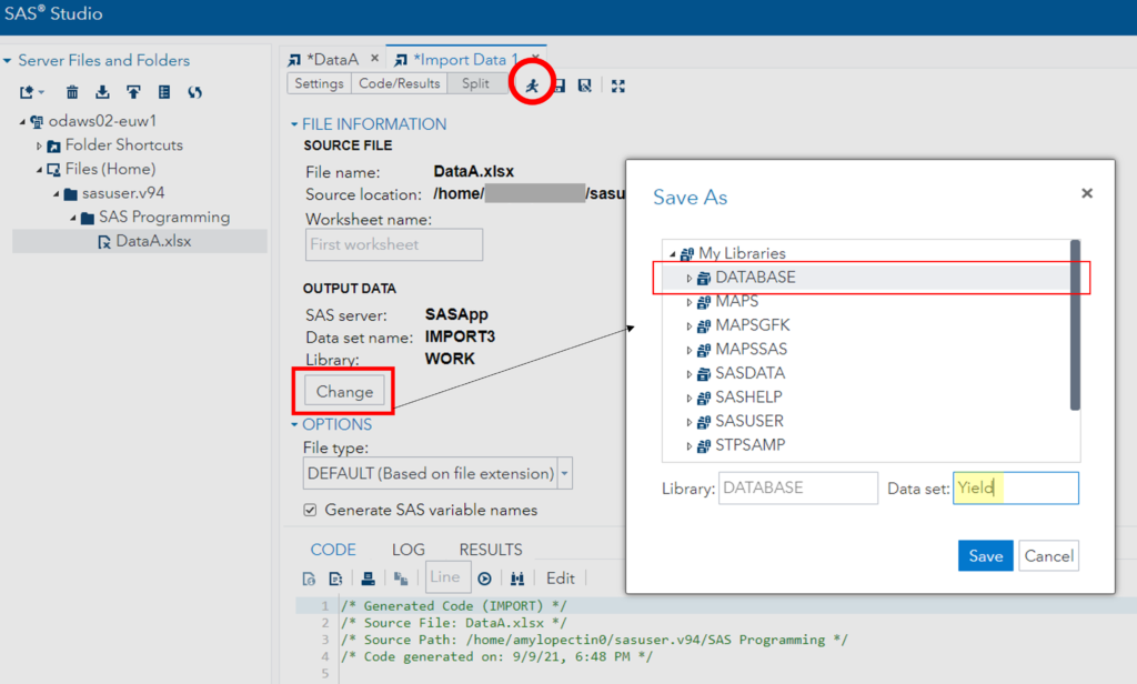
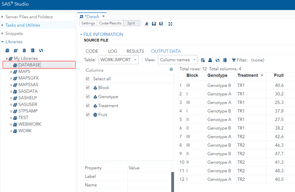
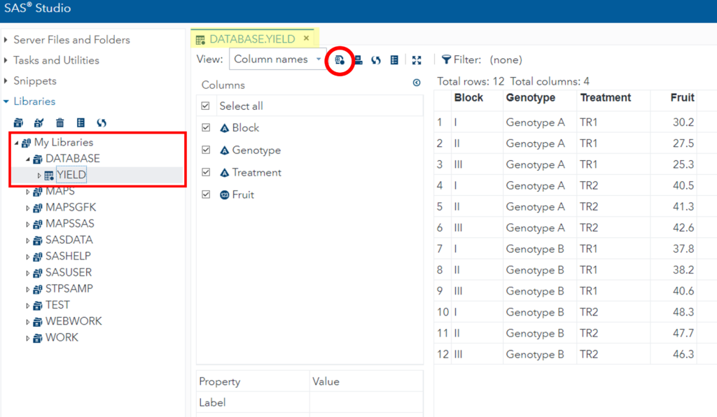
A file named ‘yield.sas7bdat’ should now appear in the ‘SAS Programming’ folder. If you navigate to the ‘DATABASE’ in My Libraries, you will find that a data table named ‘YIELD’ has been created.”

Now that the data table is within the Library, you can proceed with statistical analysis.

---

---

3. Simple statistical analysis.”

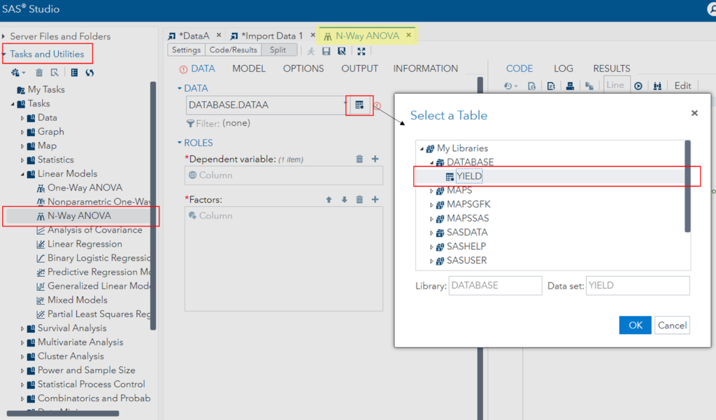
This time, select Tasks and Utilities from the left menu. Then, under ‘Linear Models,’ choose ‘N-Way ANOVA.’ A new tab for N-Way ANOVA will appear. In the ‘DATA’ section, select the ‘Yield’ data table from the Library you created.”

Now, you need to select the dependent variable (y value) and the experimental factors. For the ‘Dependent variable,’ choose ‘Fruit,’ and for the ‘Factors’ (independent variables), select ‘Block,’ ‘Genotype,’ and ‘Treatment’ all together.

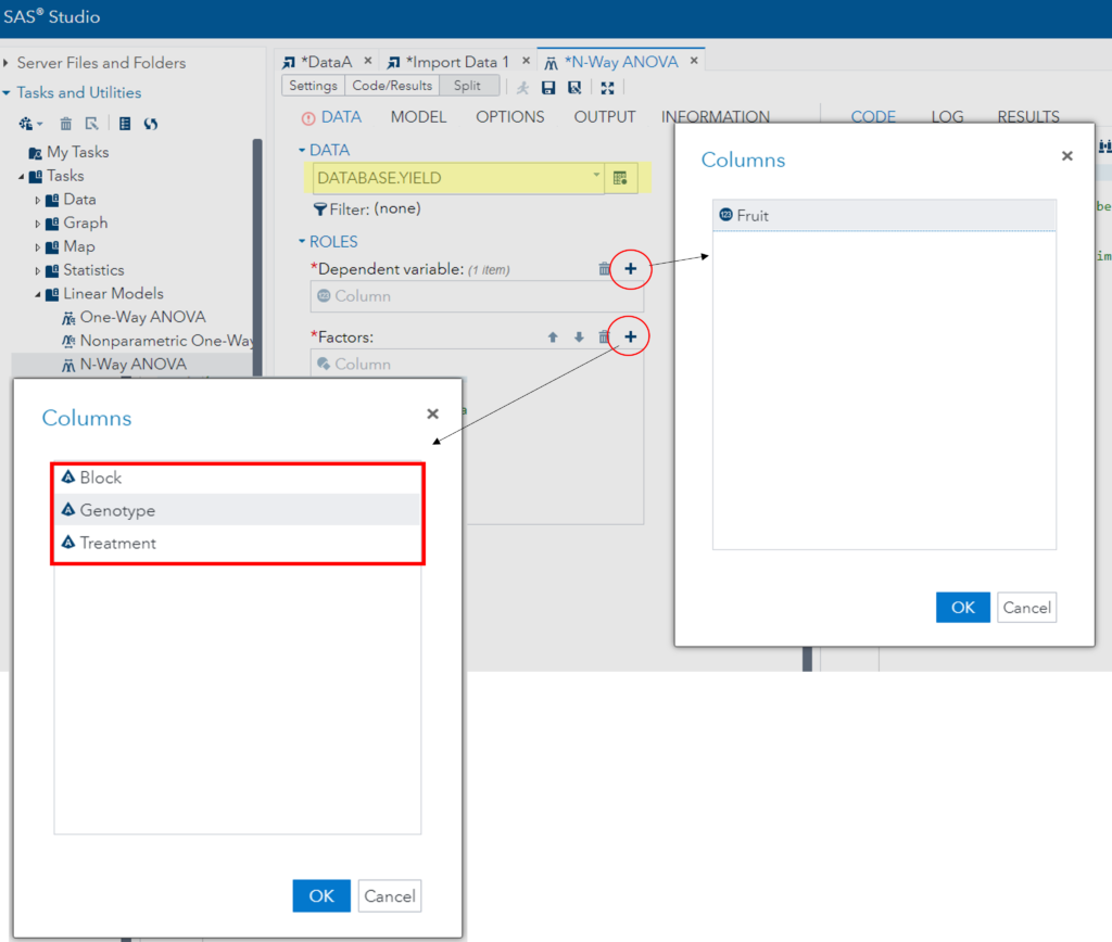
An important consideration here is that ‘Block’ should be composed of nominal values. For example, ‘Block’ should be represented as A, B, C, or I, II, III, rather than using numeric values like 1, 2, 3. If you input ‘Block’ as numeric values (1, 2, 3), when selecting the ‘Dependent variable,’ both ‘Fruit’ and ‘Block’ will appear. In this case, ‘Block’ will be recognized as a numeric variable. Consequently, if you select all three factors ‘Block,’ ‘Genotype,’ and ‘Treatment,’ ‘Block’ will not be treated as a repeated factor, but as a covariate. To avoid this issue, it’s important to input nominal values as text instead of numbers when dealing with such factors.”

---

□ What is ANCOVA (1/3)? The basic concept

---

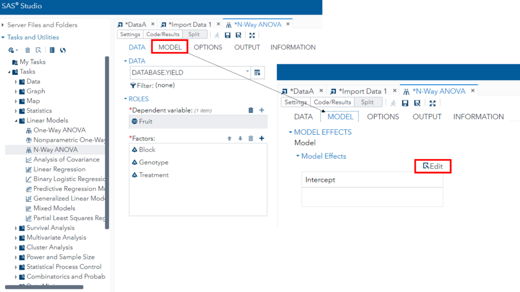
Now, let’s proceed to set up the ‘Model Effects.’ Click on ‘Edit’ under ‘MODEL.’ You want to examine how fruit weight changes based on the interaction between two factors: ‘Genotype’ and ‘Treatment.’ To do this, select both ‘Genotype’ and ‘Treatment,’ and then click Full Factorial.

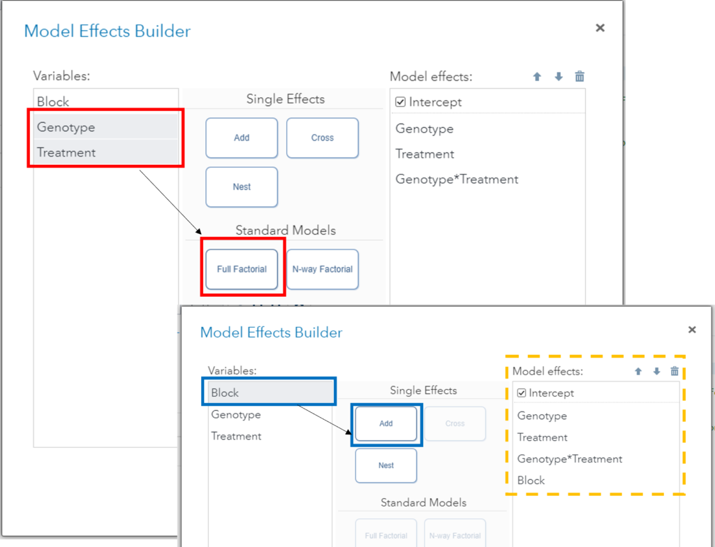
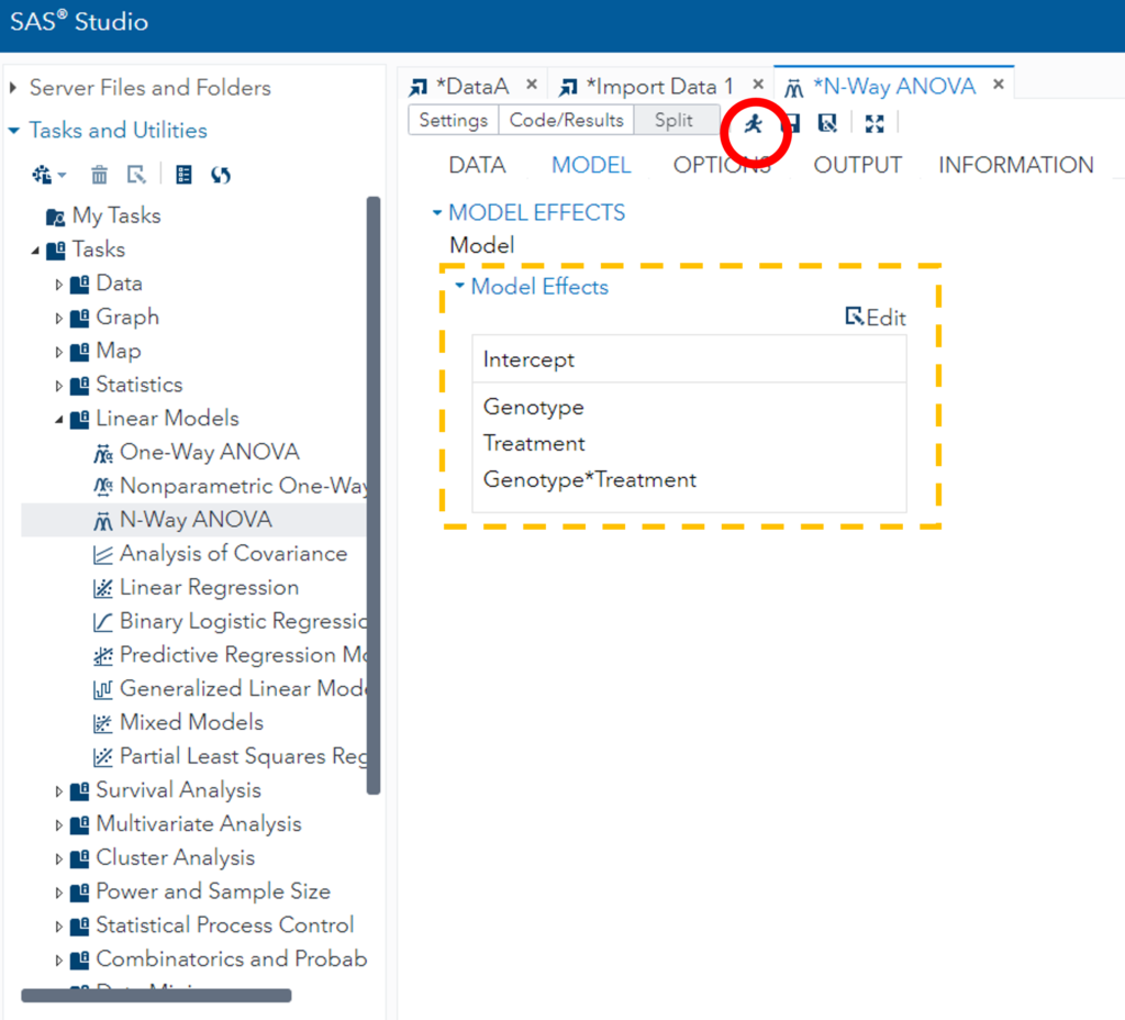
“Furthermore, since you’ve designated ‘Block’ as the repeated factor, include ‘Block’ in the model as well. As a result, the model will be composed of ‘Genotype,’ ‘Treatment,’ ‘Genotype*Treatment,’ and ‘Block.’

In statistical terms, this is a 2-Way ANOVA with a repeated measures factor (Block). The statistical model can be expressed as follows:”

yijk = μ  + αi + βj + δij + γk + εijk
yijk = 처리 (ij, i=cultivar, j=nitrogen) 및 반복에 따른 각각의 수확량 값
μ = 수확량의 전체 평균값
αi = cultivar (i) 효과
βj= Treatment (j) 효과
δij = cultivar (i) x Treatment(j) 상호작용시 효과
γk = 블록효과
εijk = 오차 

---

□ Easy-to-Understand Guide to Factorial Experiments and Two-Way ANOVA

---

---

Now that the model setup is complete, let’s proceed by clicking on ‘Run’.

Statistical results have been generated. Clicking on the code will display the code for the Block-based 2-Way ANOVA analysis.

---

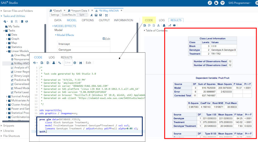
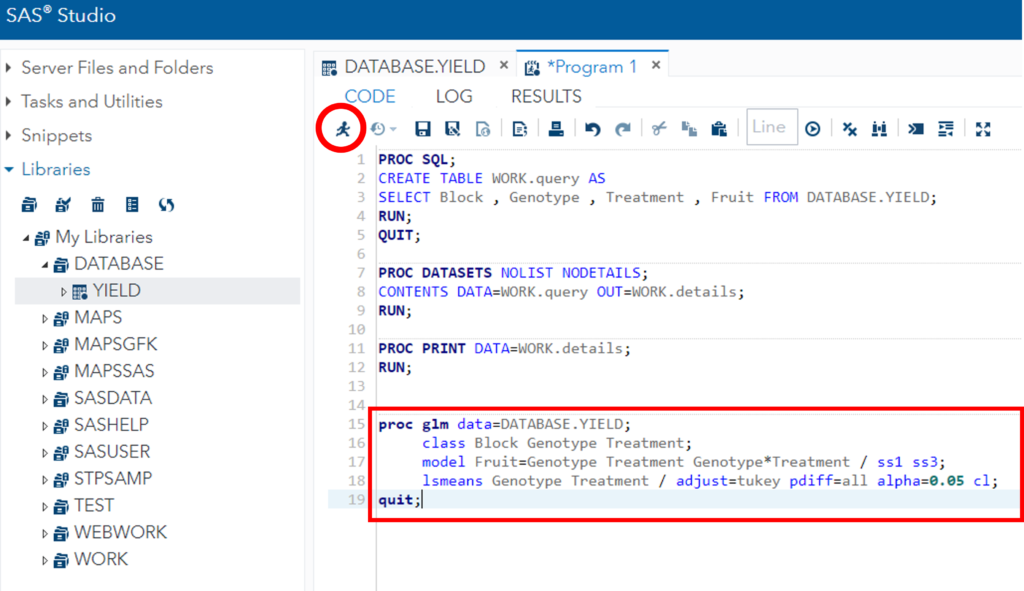
proc glm data=DATABASE.YIELD;
	 class Block Genotype Treatment;
	 model Fruit=Genotype Treatment Genotype*Treatment / ss1 ss3;
	 lsmeans Genotype Treatment / adjust=tukey pdiff=all alpha=0.05 cl;
quit;

Next time you want to perform statistical analysis, you can simply copy and paste this code.

Now, let’s clear all the steps and return to the beginning. If you want to perform ANOVA analysis again, select the YIELD data table from the Library. Then, click on the icon with a red circle. This icon generates the code.

Upon doing so, a new tab named ‘Program 1’ will appear, displaying the default code to import this data table. Below this code, you can copy and paste the ANOVA analysis code that you had previously used. Then, click the ‘Run’ button again.

Indeed, now you can get the ANOVA analysis results without the need to manually click and select each step. The process is streamlined for efficient analysis.

---

---