---

After creating a graph using R, repeatedly copying and pasting it to move it becomes a cumbersome task. Today, I’ll demonstrate how to easily relocate the graph.

Let’s generate some data and draw a graph to demonstrate.

# to generate data
title1= c("tr1","tr2","tr3")
case1x= c(3,10,17)
case1y= c(8,8,8)
case1= data.frame (title1,case1x,case1y)

# to create a graph 
library(ggplot2)
ggplot(data=case1) +
  geom_point (aes(x=case1x,y=case1y, fill=title1, shape=title1), col="Black", size=7, stroke = 0.5) +
  scale_shape_manual(values = c(21, 21, 21)) +
  scale_fill_manual(values = c("Red","Black","Dark green")) +
  scale_x_continuous(breaks = seq(0,20,5), limits = c(0,20)) +
  scale_y_continuous(breaks = seq(0,15,5), limits = c(0,15)) +
  labs(x="Treatment", y="Average grain weight") +
  theme(legend.position=c(0.90,0.9),,
        legend.title=element_blank(),
        legend.key.size=unit(0.5,'cm'),
        legend.key=element_rect(color=alpha("white",.05), 
                                fill=alpha("white",.05)),
        legend.text=element_text(size=11),
        legend.background= element_rect(fill=alpha("white",.05)),
        panel.grid.major=element_line(colour="grey90", linewidth=0.5),
        axis.line=element_line(linewidth=0.5, colour="black"))

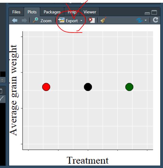
Running the code like this will display the graph in the Plot window. Then, each time, you’ll need to click Export, save it with a different name, or copy the image to place the graph where you want.

In reality, this task is quite cumbersome and becomes irritating due to its repetitive and straightforward nature. Therefore, I would like to extract graphs more easily. I will introduce two methods for achieving this.

---

---

1) using Window()

The first method involves using the windows().

library(ggplot2)
ggplot(data=case1) +
  geom_point (aes(x=case1x,y=case1y, fill=title1, shape=title1), col="Black", size=7, stroke = 0.5) +
  scale_shape_manual(values = c(21, 21, 21)) +
  scale_fill_manual(values = c("Red","Black","Dark green")) +
  scale_x_continuous(breaks = seq(0,20,5), limits = c(0,20)) +
  scale_y_continuous(breaks = seq(0,15,5), limits = c(0,15)) +
  labs(x="Treatment", y="Average grain weight") +
  theme(legend.position=c(0.90,0.9),,
        legend.title=element_blank(),
        legend.key.size=unit(0.5,'cm'),
        legend.key=element_rect(color=alpha("white",.05), 
                                fill=alpha("white",.05)),
        legend.text=element_text(size=11),
        legend.background= element_rect(fill=alpha("white",.05)),
        panel.grid.major=element_line(colour="grey90", linewidth=0.5),
        axis.line=element_line(linewidth=0.5, colour="black"))+
windows(width=5.5, height=4)

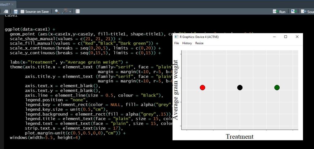
By adding windows(width=5.5, height=4) at the end of the code, you can specify the width and height, causing the graph image to appear in a new window outside the R interface. By the way, the units are in inches.

Copying and pasting this window allows for easy movement of the graph to the desired location. However, at some point, this also becomes cumbersome. You might prefer a situation where you’ve fixed the positions in a Word document and simply switch the image files while inserting graphs. In such cases, the aforementioned method would require manual copying and pasting, along with individually adjusting positions in Word. Consequently, there might arise a situation where you want to pre-save multiple graph image files and sequentially insert them.

---

---

2) using ggsave()

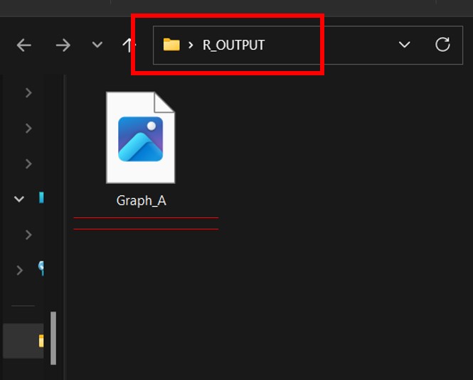
The second method involves using the ggsave() to directly save the image file. First, create a folder named “R_OUTPUT” on your desktop. The path to that folder would be something like C:/Users/Username/Desktop/R_OUTPUT. Now, let’s write the same code as before, but this time we’ll assign that code to a variable named “Fig.1”.

Fig.1= ggplot(data=case1) +
  geom_point (aes(x=case1x,y=case1y, fill=title1, shape=title1), col="Black", size=7, stroke = 0.5) +
  scale_shape_manual(values = c(21, 21, 21)) +
  scale_fill_manual(values = c("Red","Black","Dark green")) +
  scale_x_continuous(breaks = seq(0,20,5), limits = c(0,20)) +
  scale_y_continuous(breaks = seq(0,15,5), limits = c(0,15)) +
  labs(x="Treatment", y="Average grain weight") +
  theme(legend.position=c(0.90,0.9),,
        legend.title=element_blank(),
        legend.key.size=unit(0.5,'cm'),
        legend.key=element_rect(color=alpha("white",.05), 
                                fill=alpha("white",.05)),
        legend.text=element_text(size=11),
        legend.background= element_rect(fill=alpha("white",.05)),
        panel.grid.major=element_line(colour="grey90", linewidth=0.5),
        axis.line=element_line(linewidth=0.5, colour="black"))

Then, use the ggsave() to save the graph image assigned to variable “Fig.1” to the specified path. You can also specify the width, height, and resolution (dpi). When saving the image, I’ll impose the name as Graph_A

ggsave("C:/Users/Username/Desktop/R_OUTPUT/Graph_A.jpg", Fig.1, width= 12.5, height= 10, units= "cm", dpi= 1000)

As a result, the file will be saved directly to the “R_OUTPUT” folder. When using the ggsave(), the graph image might not be immediately visible, meaning you would need to open the saved image file to view the graph. Therefore, the method I frequently use is as follows.

Fig.1= ggplot(data=case1) +
  geom_point (aes(x=case1x,y=case1y, fill=title1, shape=title1), col="Black", size=7, stroke = 0.5) +
  scale_shape_manual(values = c(21, 21, 21)) +
  scale_fill_manual(values = c("Red","Black","Dark green")) +
  scale_x_continuous(breaks = seq(0,20,5), limits = c(0,20)) +
  scale_y_continuous(breaks = seq(0,15,5), limits = c(0,15)) +
  labs(x="Treatment", y="Average grain weight") +
  theme(legend.position=c(0.90,0.9),,
        legend.title=element_blank(),
        legend.key.size=unit(0.5,'cm'),
        legend.key=element_rect(color=alpha("white",.05), 
                                fill=alpha("white",.05)),
        legend.text=element_text(size=11),
        legend.background= element_rect(fill=alpha("white",.05)),
        panel.grid.major=element_line(colour="grey90", linewidth=0.5),
        axis.line=element_line(linewidth=0.5, colour="black"))

Fig.1 + windows(width=5.5, height=4)

ggsave("C:/Users/Username/Desktop/R_OUTPUT/Graph_A.jpg", Fig.1, width= 12.5, height= 10, units= "cm", dpi= 1000)

I start by using the windows() function to preview the graph. If there are any modifications needed, I directly go to the ggplot code to make the changes. Once the graph is finalized, I save it as the final image file. When writing the ggplot code, incorporating both the windows() function and the ggsave() function provides the advantage of real-time graph modification and immediate saving to image files.

---

---