---

Sometimes, we need to insert a linear regression equation inside a graph, but it’s an annoying to type an equation every time when generating a linear regression graph. Using stat_poly_eq(), we can automatically insert a linear regression equation.

Let’s generate one data frame.

x= c(1, 2, 3, 4, 5, 6, 7)
y= c(10, 13, 15, 14, 16, 19, 20)
dataA= data.frame (x, y)

Then, I’ll generate a regression graph.

if(!require(ggplot2)) install.packages("ggplot2")
library(ggplot2)

ggplot(data=dataA, aes(x=x, y=y)) +
  geom_point(size=1.5, stroke=1) +
  geom_smooth(method=lm, level=0.95, se=TRUE, linetype=1, size=0.5, formula=y~x) +
  scale_x_continuous(breaks=seq(0,10,2), limits=c(0,10)) +
  scale_y_continuous(breaks=seq(0,20,5), limits=c(0,20)) +
  labs(x="Weight", y="Height") +
  theme_classic(base_size= 15, base_family = "serif") +
  theme(legend.position="none",
        legend.title=element_blank(),
        legend.key=element_rect(color="white", fill=alpha(0.5)),
        legend.text=element_text(family="serif", face="plain",
                                 size=15, color="black"),
        legend.background= element_rect(fill=alpha(0.5)),
        axis.line= element_line(linewidth= 0.5, colour= "black")) +
  windows(width=6, height=5.5)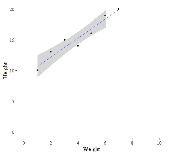

Now let’s analyze a linear regression.

Regression= lm (y ~ x, data=dataA)
summary (Regression) 

Coefficients:
            Estimate Std. Error t value Pr(>|t|)    
(Intercept)   9.1429     0.8777  10.416 0.000141 ***
x             1.5357     0.1963   7.825 0.000547 ***
---
Signif. codes:  0 ‘***’ 0.001 ‘**’ 0.01 ‘*’ 0.05 ‘.’ 0.1 ‘ ’ 1

Residual standard error: 1.039 on 5 degrees of freedom
Multiple R-squared:  0.9245,	Adjusted R-squared:  0.9094 
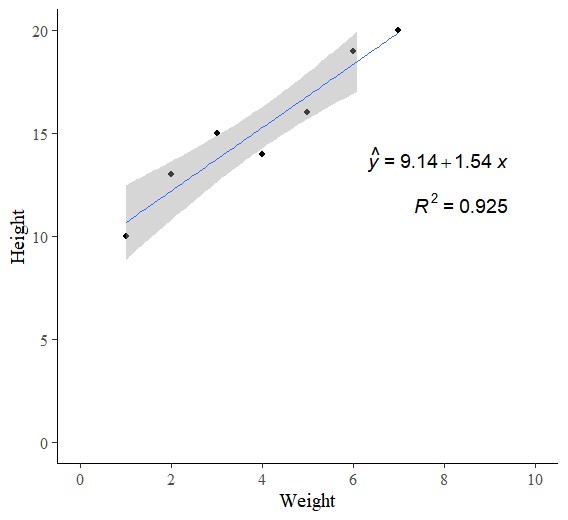
F-statistic: 61.23 on 1 and 5 DF,  p-value: 0.0005468

The linear model equation is y= 9.1429 + 1.5357x and R² is 0.9245. Now I’ll insert this equation model automatically using stat_poly_eq(). I’ll add the below codes.

if (require("ggpmisc") == F) install.packages("ggpmisc")
library(ggpmisc)

ggplot(data=dataA, aes(x=x, y=y)) +
geom_point(size=1.5, stroke = 1) +
geom_smooth(method=lm, level=0.95, se=TRUE, linetype=1, size=0.5, formula=y~x) +
#Equation
 stat_poly_eq(aes(label= paste(..eq.label.., sep= "~~~")),
              label.x=0.9, label.y=0.7,
              eq.with.lhs= "italic(hat(y))~'='~", eq.x.rhs= "~italic(x)",
              coef.digits=3, formula=y ~ x, parse=TRUE, size=5)+
# R-squared
 stat_poly_eq(aes(label=paste(..rr.label.., sep= "~~~")),
              label.x=0.9, label.y=0.6, rr.digits=3,
              formula=y ~ x, parse=TRUE, size=5) +
scale_x_continuous(breaks=seq(0,10,2), limits=c(0,10)) +
scale_y_continuous(breaks=seq(0,20,5), limits=c(0,20)) +
labs(x="Weight", y="Height") +
  theme_classic(base_size= 15, base_family = "serif") +
  theme(legend.position="none",
        legend.title=element_blank(),
        legend.key=element_rect(color="white", fill=alpha(0.5)),
        legend.text=element_text(family="serif", face="plain",
                                 size=15, color="black"),
        legend.background= element_rect(fill=alpha(0.5)),
        axis.line= element_line(linewidth= 0.5, colour= "black")) +
  windows(width=6, height=5.5)

Then, the equation is inserted automatically inside the graph.

# full code
ggplot(data=data.frame (c(1, 2, 3, 4, 5, 6, 7), c(10, 13, 15, 14, 16, 19, 20)), 
       aes(x=x, y=y)) +
  geom_point(size=1.5, stroke = 1) +
  geom_smooth(method=lm, level=0.95, se=TRUE, linetype=1, size=0.5, formula=y~x) +

  #Equation
  stat_poly_eq(aes(label= paste(..eq.label.., sep= "~~~")),
               label.x=0.9, label.y=0.7,
               eq.with.lhs= "italic(hat(y))~'='~", eq.x.rhs= "~italic(x)",
               coef.digits=3, formula=y ~ x, parse=TRUE, size=5)+
  # R-squared
  stat_poly_eq(aes(label=paste(..rr.label.., sep= "~~~")),
               label.x=0.9, label.y=0.6, rr.digits=3,
               formula=y ~ x, parse=TRUE, size=5)+
  
  scale_x_continuous(breaks=seq(0,10,2), limits=c(0,10)) +
  scale_y_continuous(breaks=seq(0,20,5), limits=c(0,20)) +
  labs(x="Weight", y="Height") +
  theme_classic(base_size= 15, base_family = "serif") +
  theme(legend.position="none",
        legend.title=element_blank(),
        legend.key=element_rect(color="white", fill=alpha(0.5)),
        legend.text=element_text(family="serif", face="plain",
                                 size=15, color="black"),
        legend.background= element_rect(fill=alpha(0.5)),
        axis.line= element_line(linewidth= 0.5, colour= "black")) +
  windows(width=6, height=5.5)

---

We aim to develop open-source code for agronomy (kimjk@agronomy4future.com)