What is Finlay-Wilkinson Regression Model?
The genotype is dependent on environmental changes. One genotype may strongly respond to certain environmental conditions, while another genotype may weakly respond to the same conditions. If some genotypes strongly respond under better conditions, they would be adaptable to the environment.
Adaptability refers to the flexibility of a genotype in its response to improved environments.
If a certain genotype exhibits high performance across a wide range of environmental conditions, it would be considered to have broad adaptation.
To achieve this definition, two prerequisites are required.
- In general, greater performances
- Less variation across environmental ranges
I’ll create one dataset.
Env= c("High_inoc","High_NO_inoc","Low_inoc", "Low_NO_inoc")
CV1= c(30,150,20,100)
CV2= c(74,99,49,73)
CV3= c(78,106,56,69)
CV4= c(86,92,66,70)
CV5= c(74,98,57,79)
Data= data.frame(Env,CV1,CV2,CV3,CV4,CV5)
Data

Env	        CV1	CV2	CV3	CV4	CV5
High_inoc	30	74	78	86	74
High_NO_inoc	150	99	106	92	98
Low_inoc	20	49	56	66	57
Low_NO_inoc	100	73	69	70	79
There are five different genotypes (CV1 – CV5), and each genotype was subjected to four different treatments. Let’s assume that the combination of organic matter and virus inoculation was applied to each genotype to observe the differences in final yield.
High_inoc: High organic matter + virus inoculation
High_NO_inoc: High organic matter + virus free
Low_inoc: Low organic matter + virus inoculation
Low_NO_inoc : Low organic matter + virus free
Which treatment would affect yield the most negatively? Maybe under the low organic matter and inoculation (the worst condition), the yield would be the lowest.
Let’s see it’s true.
library(dplyr)
Data$Mean= rowMeans (Data %>% select(-Env))
Data= rbind(Data, c("Mean", colMeans(Data %>% select(-Env))))

Data
Env	        CV1	CV2	CV3	CV4	CV5	Mean
High_inoc	30	74	78	86	74	68.4
High_NO_inoc	150	99	106	92	98	109.0
Low_inoc	20	49	56	66	57	49.6
Low_NO_inoc	100	73	69	70	79	78.2
Mean	        75.0	73.75	77.25	78.5	77.0	76.3
We can calculate two different averages: each genotype across treatments, and each treatment (or environment) across genotypes. As we assumed, the condition of low organic matter and inoculation (Low_inoc) showed the lowest yield (49.6). For genotype, CV4 showed the greatest yield across treatments (78.5).
So, is it okay to say that CV4 is the best cultivar for yield? It would be the best cultivar for yield as it shows the greatest yield across environmental conditions. However, let’s focus on the worst condition (Low_inoc). If CV4 is the best cultivar, it should also show the greatest yield in Low_inoc. However, it seems not because it is 66 in Low_inoc, showing the lowest yield. As mentioned above, the average of Low_inoc was 49.6, and CV4 contributes to the lowest yield in Low_inoc. Therefore, we should not only consider yield but also adaptability when comparing genotypes across different environmental conditions.
Environmental Index will explain adaptability.
Now, I’ll calculate environmental index. This is the difference between the mean of each environment and the grand mean (X.. - X.j).
68.4 – 76.3 = -7.9
109 – 76.3 = 32.7
49.6 – 76.3 = -26.7
78.2 – 76.3 = 1.9
library(dplyr)
Data$Mean= as.numeric(Data$Mean)
Data$Env_index= Data$Mean - Data$Mean[nrow(Data)]

Data
Env       	CV1	CV2	CV3	CV4	CV5	Mean	Env_index
High_inoc	30	74	78	86	74	68.4	-7.9
High_NO_inoc	150	99	106	92	98	109.0	32.7
Low_inoc	20	49	56	66	57	49.6	-26.7
Low_NO_inoc	100	73	69	70	79	78.2	1.9
Mean	        75.0	73.75	77.25	78.5	77.0	76.3	0.0
I calculated the environmental index for four different environmental conditions. As expected, at Low_inoc (low organic matter + virus inoculation), it shows the lowest environmental index (-26.7). Conversely, at High_NO_inoc (high organic matter + virus-free), it shows the highest environmental index (32.7).
Environmental Index will be independent variable in linear regression.
Now, each genotype will be fitted by linear regression. Of course, yield will be the dependent variable (y). Then, what would be the independent variable (x) in the regression model? In the Finlay-Wilkinson Regression Model, the environmental index becomes the independent variable (x). Therefore, the environmental index should be stacked in rows.
First, I’ll delete the mean I calculated.
Data= Data [-5,-7]  # delete 5th row and 7th column

Data
           Env CV1 CV2 CV3 CV4 CV5 Env_index
1    High_inoc  30  74  78  86  74      -7.9
2 High_NO_inoc 150  99 106  92  98      32.7
3     Low_inoc  20  49  56  66  57     -26.7
4  Low_NO_inoc 100  73  69  70  79       1.9
Then, I’ll stack data in rows using the below code.
library(tidyr)
df= data.frame(
               Data %>%
               pivot_longer(
               cols=c(CV1, CV2, CV3, CV4, CV5),
               names_to="Genotype", values_to="Yield")
               )

df
Env	     Env_index	Genotype Yield
High_inoc	-7.9	CV1	 30
High_inoc	-7.9	CV2	 74
High_inoc	-7.9	CV3	 78
High_inoc	-7.9	CV4	 86
High_inoc	-7.9	CV5	 74
High_NO_inoc	32.7	CV1	 150
.
.
.
Now I’ll fit each genotype with an environmental index using the code below.
if(!require(dplyr)) install.packages("dplyr")
library(dplyr)

summary(lm (Yield ~ Env_index, data=dataA %>% filter (Genotype=="CV1")))
summary(lm (Yield ~ Env_index, data=dataA %>% filter (Genotype=="CV2")))
summary(lm (Yield ~ Env_index, data=dataA %>% filter (Genotype=="CV3")))
summary(lm (Yield ~ Env_index, data=dataA %>% filter (Genotype=="CV4")))
summary(lm (Yield ~ Env_index, data=dataA %>% filter (Genotype=="CV5")))
or
regression= dataA%>% group_by(Genotype) %>% do(model= lm(Yield~Env_index, data=.))

regression$model

[[1]]
Call:
lm(formula = Yield ~ Env_index, data = .)

Coefficients:
(Intercept)    Env_index
      75.00         2.34

[[2]]
Call:
lm(formula = Yield ~ Env_index, data = .)

Coefficients:
(Intercept)    Env_index
    73.7500       0.8025

[[3]]
Call:
lm(formula = Yield ~ Env_index, data = .)

Coefficients:
(Intercept)    Env_index
     77.250        0.804

[[4]]
Call:
lm(formula = Yield ~ Env_index, data = .)

Coefficients:
(Intercept)    Env_index
    78.5000       0.3786

[[5]]
Call:
lm(formula = Yield ~ Env_index, data = .)

Coefficients:
(Intercept)    Env_index
    77.0000       0.6754
However, I recommend using the following code.
if(!require(broom)) install.packages("broom")
library(broom)

regression1= df %>% group_by(Genotype) %>% do(tidy(lm(Yield ~ Env_index, data=.)))

regression1
Genotype	term	estimate	std.error	statistic	p.value
CV1	(Intercept)	75.0000000	12.1638994	6.165786	0.025309723
CV1	Env_index	2.3395736	0.5658852	4.134361	0.053823885
CV2	(Intercept)	73.7500000	2.7528814	26.790112	0.001390415
CV2	Env_index	0.8024564	0.1280687	6.265828	0.024537235
CV3	(Intercept)	77.2500000	4.3607461	17.714859	0.003171427
CV3	Env_index	0.8039714	0.2028693	3.963002	0.058171978
CV4	(Intercept)	78.5000000	5.0252942	15.620976	0.004073090
CV4	Env_index	0.3786387	0.2337852	1.619601	0.246746749
CV5	(Intercept)	77.0000000	1.1734503	65.618456	0.000232165
CV5	Env_index	0.6753598	0.0545909	12.371290	0.006470516
Now, let’s focus on the slope of the regression in each genotype. Which genotype shows the steepest slope? It’s CV1 (2.34).
The model equation of CV1 is y = 75.0 + 2.317 * Env_Index. This means that when the environmental index increases by 1, yield will increase by 2.317 times.
For a clearer visualization, I’ll draw a regression graph.
library(ggplot2)
ggplot(data=df, aes(x=as.numeric(Env_index), y=as.numeric(Yield), group=Genotype)) +
  geom_smooth(method = lm, level=0.95, se=FALSE, linetype=1, color="Dark red",
              linewidth=0.5, formula= y ~ x) +
  geom_point (aes(shape=Genotype, fill=Genotype), col="Black", size=5, stroke = 0.5) +
  scale_shape_manual(values = c(21, 22, 23, 24, 25)) +
  scale_fill_manual(values = c("Black","Red",'Blue',"Orange","Green")) +
  scale_x_continuous(breaks = seq(-40,40,10), limits = c(-40,40)) +
  scale_y_continuous(breaks = seq(0,200,20), limits = c(0,200)) +
  labs(x="Environmental Index", y="Yield") +
  theme_classic(base_size=18, base_family="serif")+
  theme(legend.position=c(0.89,0.17),
        legend.title=element_blank(),
        legend.key=element_rect(color="white", fill="white"),
        legend.text=element_text(family="serif", face="plain",
                                 size=15, color= "Black"),
        legend.background=element_rect(fill="white"),
        axis.line=element_line(linewidth=0.5, colour="black"))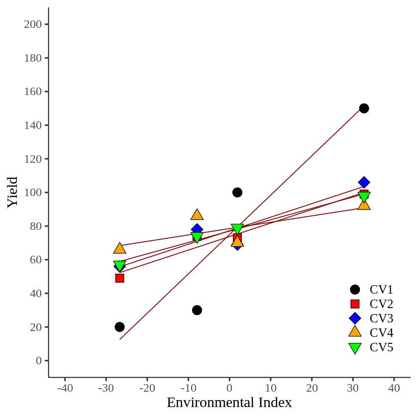
Now it’s much clear. CV1 shows the steepest slope among genotypes. If we consider only yield across environmental conditions, CV4 showed the greatest yield, but it shows less slope than CV1.
CV1: y=75.0 + 2.317 * Env_Index
CV4: y=78.5 + 0.374 * Env_Index
Therefore, in terms of adaptability, we might be able to say CV4 is the best cultivar. That is, in Finlay-Wilkinson Regression Model, CV4 would have the greatest environmental adaptability.
full code: https://github.com/agronomy4future/r_code/blob/main/What_is_Finlay_Wilkinson_Regression_Model.ipynb
The model equation of Finlay-Wilkinson regression
p = G + βE + e

where
G is intercept (genotypic effect)
β is slope (sensitivity to environment; adaptability))
e is error
In this post, I explained how to obtain β.
When we analyze our field data across environmental conditions, β would provide many more insights about our crops. Particularly, when we analyze genotypes under multi-environmental trials (METs), the Finlay-Wilkinson regression would be very useful to understand how genotypes respond to environments.
■ fwrmodel() package
Github: https://github.com/agronomy4future/fwrmodel
To easily calculate the environmental index, I recently developed an R package called fwrmodel(). I will use the same data mentioned above to calculate the environmental index.
Env= c("High_inoc","High_NO_inoc","Low_inoc", "Low_NO_inoc")
CV1= c(30,150,20,100)
CV2= c(74,99,49,73)
CV3= c(78,106,56,69)
CV4= c(86,92,66,70)
CV5= c(74,98,57,79)
Data= data.frame(Env,CV1,CV2,CV3,CV4,CV5)

Env	        CV1	CV2	CV3	CV4	CV5
High_inoc	30	74	78	86	74
High_NO_inoc	150	99	106	92	98
Low_inoc	20	49	56	66	57
Low_NO_inoc	100	73	69	70	79
First, we need to transpose the dataset as shown below
if(!require(dplyr)) install.packages("dplyr")
if(!require(tidyr)) install.packages("tidyr")
library(dplyr)
library(tidyr)

dataA= data.frame(Data %>%
       pivot_longer(
       cols= c(CV1,CV2,CV3,CV4,CV5),
       names_to= "Cultivar",
       values_to= "Yield"))

dataA
            Env Cultivar Yield
1     High_inoc      CV1    30
2     High_inoc      CV2    74
3     High_inoc      CV3    78
4     High_inoc      CV4    86
5     High_inoc      CV5    74
6  High_NO_inoc      CV1   150
7  High_NO_inoc      CV2    99
8  High_NO_inoc      CV3   106
9  High_NO_inoc      CV4    92
10 High_NO_inoc      CV5    98
11     Low_inoc      CV1    20
12     Low_inoc      CV2    49
13     Low_inoc      CV3    56
14     Low_inoc      CV4    66
15     Low_inoc      CV5    57
16  Low_NO_inoc      CV1   100
17  Low_NO_inoc      CV2    73
18  Low_NO_inoc      CV3    69
19  Low_NO_inoc      CV4    70
20  Low_NO_inoc      CV5    79
I’ll calculate the environmental index for each cultivar in relation to the environment using the fwrmodel() package.
# installation
if(!require(remotes)) install.packages("remotes")
remotes::install_github("agronomy4future/fwrmodel")
library(remotes)
library(fwrmodel)

stability= fwrmodel(df, env_cols = c("Env"),
                    genotype_col= "Cultivar", yield_cols= c("Yield"))

env_index_cal= data.frame(stability$env_index)

env_index_cal
   Cultivar          Env Environments Env_index_Yield Yield
1       CV1    High_inoc    High_inoc            -7.9    30
2       CV2    High_inoc    High_inoc            -7.9    74
3       CV3    High_inoc    High_inoc            -7.9    78
4       CV4    High_inoc    High_inoc            -7.9    86
5       CV5    High_inoc    High_inoc            -7.9    74
6       CV1 High_NO_inoc High_NO_inoc            32.7   150
7       CV2 High_NO_inoc High_NO_inoc            32.7    99
8       CV3 High_NO_inoc High_NO_inoc            32.7   106
9       CV4 High_NO_inoc High_NO_inoc            32.7    92
10      CV5 High_NO_inoc High_NO_inoc            32.7    98
11      CV1     Low_inoc     Low_inoc           -26.7    20
12      CV2     Low_inoc     Low_inoc           -26.7    49
13      CV3     Low_inoc     Low_inoc           -26.7    56
14      CV4     Low_inoc     Low_inoc           -26.7    66
15      CV5     Low_inoc     Low_inoc           -26.7    57
16      CV1  Low_NO_inoc  Low_NO_inoc             1.9   100
17      CV2  Low_NO_inoc  Low_NO_inoc             1.9    73
18      CV3  Low_NO_inoc  Low_NO_inoc             1.9    69
19      CV4  Low_NO_inoc  Low_NO_inoc             1.9    70
20      CV5  Low_NO_inoc  Low_NO_inoc             1.9    79
and let’s obtain slope (stability).
coefficient_AGW= as.data.frame(stability$regression$Yield)

coefficient_AGW
   Cultivar            term   estimate  std.error statistic     p.value
1       CV1     (Intercept) 75.0000000 12.1638994  6.165786 0.025309723
2       CV1 Env_index_Yield  2.3395736  0.5658852  4.134361 0.053823885
3       CV2     (Intercept) 73.7500000  2.7528814 26.790112 0.001390415
4       CV2 Env_index_Yield  0.8024564  0.1280687  6.265828 0.024537235
5       CV3     (Intercept) 77.2500000  4.3607461 17.714859 0.003171427
6       CV3 Env_index_Yield  0.8039714  0.2028693  3.963002 0.058171978
7       CV4     (Intercept) 78.5000000  5.0252942 15.620976 0.004073090
8       CV4 Env_index_Yield  0.3786387  0.2337852  1.619601 0.246746749
9       CV5     (Intercept) 77.0000000  1.1734503 65.618456 0.000232165
10      CV5 Env_index_Yield  0.6753598  0.0545909 12.371290 0.006470516