[R package] Finlay-Wilkinson Regression model (feat. fwrmodel)
■ What is Finlay-Wilkinson Regression Model?
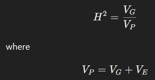
In my previous post, I introduced what Finlay-Wilkinson Regression Model is and how to calculate adaptability (or stability). Actually, adaptability and stability are opposite concept with the same data. Have you ever heard heritability (h2)? Heritability is a key concept in genetics and breeding that measures how much of the variation in a trait within a population is due to genetic differences among individuals. In other words, it quantifies the proportion of phenotypic variation (observable traits) that can be attributed to genetic factors.
High Heritability means that a large portion of the trait’s variation is due to genetic differences, suggesting that the trait is more stable and less influenced by environmental factors. This implies that the trait is less plastic, or less responsive to changes in the environment. On the other hand, low heritability indicates that environmental factors play a larger role in the variation of the trait. Traits with low heritability are more plastic, meaning they show greater variability in response to different environmental conditions.
Adaptability and stability are analogous to the inverse relationship between heritability and plasticity.
Adaptability refers to a trait’s ability to change or respond effectively to different environmental conditions. A trait with high adaptability will show significant variation in response to environmental changes. For instance, a crop variety with high adaptability may perform well across a wide range of environments, but its performance might vary significantly depending on the conditions. High adaptability generally means a trait has greater plasticity, or flexibility, to respond to environmental changes. This can be beneficial in environments that are highly variable but may come with trade-offs in terms of consistency.
On the other hand, stability reflects how consistent a trait’s performance is across varying environments. A trait with high stability will show little variation in response to different environmental conditions, indicating that it performs reliably regardless of changes in the environment. High stability indicates that a trait performs consistently across different environments, but it might not show as much variation or responsiveness to environmental changes. This can be advantageous for ensuring reliable performance but may not be as flexible in adapting to new or extreme conditions.
Therefore, the concepts of adaptability and stability are indeed complementary but inversely related: improving one can often come at the expense of the other. Understanding this trade-off is crucial in fields like crop breeding, where both adaptability and stability might be desired but need to be balanced according to specific goals and environmental contexts.
■ Quantifying Phenotypic Plasticity of Crops
To calculate adaptability or stability (hereafter referred to as stability), the first step is to calculate the environmental index.
if(!require(dplyr)) install.packages("dplyr")
library(dplyr)

Condition= c("High_inoc", "High_NO_inoc", "Low_inoc", "Low_NO_inoc")
CV= matrix(c(30, 74, 78, 86, 74, 150, 99, 106, 92, 98, 20, 49, 56, 66, 57, 100, 73, 69, 70, 79), ncol= 5, byrow= TRUE)
colnames(CV)= paste0("CV", 1:5)
df= data.frame(Condition, CV)

df$Mean= rowMeans (df %>% select(-Condition))
df= rbind(df, c("Mean", colMeans(df %>% select(-Condition))))

Env	        CV1	CV2	CV3	CV4	CV5	Mean
High_inoc	30	74	78	86	74	68.4
High_NO_inoc	150	99	106	92	98	109.0
Low_inoc	20	49	56	66	57	49.6
Low_NO_inoc	100	73	69	70	79	78.2
Mean	        75.0	73.75	77.25	78.5	77.0	76.3

df$Mean= as.numeric(df$Mean)
df$Env_index= df$Mean - df$Mean[nrow(df)]

Env       	CV1	CV2	CV3	CV4	CV5	Mean	Env_index
High_inoc	30	74	78	86	74	68.4	-7.9
High_NO_inoc	150	99	106	92	98	109.0	32.7
Low_inoc	20	49	56	66	57	49.6	-26.7
Low_NO_inoc	100	73	69	70	79	78.2	1.9
Mean	        75.0	73.75	77.25	78.5	77.0	76.3	0.0
The code provided outlines the general process for calculating the environmental index. However, most datasets we work with will not follow the structure shown above. I combined two variables—nitrogen (high or low) and virus (inoculated or non-inoculated)—into a single factor and displayed the genotypes (CV1 to CV5) horizontally. In an actual dataset, the structure would be more like the example below.
Nitrogen Virus   Genotype Yield
High     inoc    CV1      30
High     inoc    CV2      74
High     inoc    CV3      78
High     inoc    CV4      86
High     inoc    CV5      74
High     noinoc  CV1      150
High     noinoc  CV2      99
High     noinoc  CV3      106
High     noinoc  CV4      92
High     noinoc  CV5      98
Low      inoc    CV1      20
Low      inoc    CV2      49
Low      inoc    CV3      56
Low      inoc    CV4      66
Low      inoc    CV5      57
Low      noinoc  CV1      100
Low      noinoc  CV2      73
Low      noinoc  CV3      69
Low      noinoc  CV4      70
High     noinoc  CV5      79
In this case, we need to reorganize the dataset and calculate the environmental index step by step.
■ fwrmodel() package
To solve this program, recently I developed R package to calculate environmental index and stability simultaneously. It’s fwrmodel() package.
Github: https://github.com/agronomy4future/fwrmodel
Let’s upload one dataset.
if(!require(readr)) install.packages("readr")
library(readr)
github="https://raw.githubusercontent.com/agronomy4future/raw_data_practice/main/fwrm_package_data_practice.csv"
df= data.frame(read_csv(url(github), show_col_types=FALSE))

set.seed(100)
df[sample(nrow(df),5),]
    year variety nitrogen location   AGW   KN      GY
202 2023     cv2       N0 Nebraska 318.6 3764 11864.8
112 2024     cv2       N1     Iowa 313.6 4570 14177.8
206 2023     cv2       N0 Nebraska 338.9 3764 12619.8
4   2023     cv1       N1     Iowa 311.7 3476 10721.4
98  2024     cv1       N1     Iowa 263.9 5618 14669.2
.
.
.
Let’s assume this data represents grain weight (AGW), grain number per m² (KN), and grain yield (kg/ha, GY) of corn across different states in the U.S. for two different seasons. I want to calculate the stability of each yield component and grain yield to determine which genotypes show better stability for AGW, KN, and GY, respectively.
First, I’ll install the package, but before that, it’s necessary to install Rtools because my package was developed outside of CRAN.
https://cran.r-project.org/bin/windows/Rtools
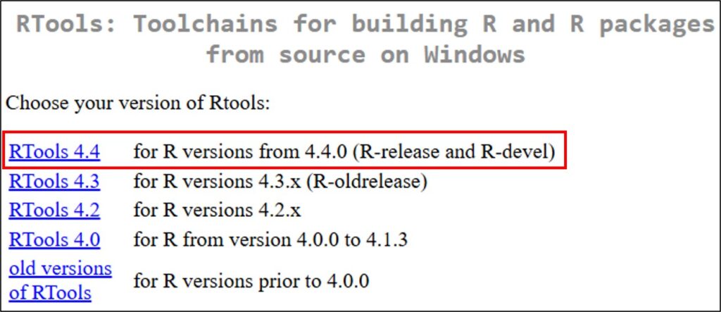
Please install the version corresponding to your current R version, and install the fwrmodel() package as the following code.
if(!require(remotes)) install.packages("remotes")
remotes::install_github("agronomy4future/fwrmodel")

library(remotes)
library(fwrmodel)
and I’ll run the code as shown below to calculate the environmental index.
stability= fwrmodel(df, env_cols = c("year", "nitrogen", "location"),
                    genotype_col= "variety", yield_cols= c("AGW","GY","KN"))

env_index_cal= data.frame(stability$env_index)
set.seed(100)
env_index_cal[sample(nrow(env_index_cal),5),]
variety year nitrogen location Environments Env_index_AGW AGW Env_index_GY GY Env_index_KN KN
20170 cv2 2023 N0 Nebraska 2023_N0_Nebraska 3.443333 318.6 -435.7763 11810.8 -214.5600 3488
16887 cv1 2023 N0 Illinois 2023_N0_Illinois -1.523333 307.0 -2300.4197 8130.4 -786.9267 2742
3430 cv2 2023 N1 Iowa 2023_N1_Iowa -22.023333 337.4 -202.7063 11931.9 195.4400 3721
3696 cv2 2023 N1 Iowa 2023_N1_Iowa -22.023333 289.0 -202.7063 10474.6 195.4400 3411
20474 cv2 2023 N0 Nebraska 2023_N0_Nebraska 3.443333 348.8 -435.7763 10947.9 -214.5600 3672I want to calculate the environmental index for AGW, KN, and GY across year, nitrogen, and location, respectively. The code to do this is as shown above.
Note 1
Setting up environments to calculate environmental index is important because it directly affects stability (slope). For example, if you think the year is not an important factor for crop yield in this case, you might combine environments with only nitrogen and location. This could result in a completely different slope for each genotype. Therefore, the most important thing is to understand your own dataset and determine the best combination of environments to calculate stability.
Next, I’ll calculate stability.
coefficient_AGW= as.data.frame(stability$regression$AGW)
coefficient_KN= as.data.frame(stability$regression$KN)
coefficient_GY= as.data.frame(stability$regression$GY)
Let’s check the coefficient for AGW.
print(coefficient_AGW)
  variety          term    estimate  std.error  statistic  p.value
1     cv1   (Intercept) 297.9520000 3.95194803  75.393704  1.368777e-88
2     cv1 Env_index_AGW   0.7523172 0.14292608  5.263681   8.336224e-07
3     cv2   (Intercept) 318.8220000 2.58702388  123.238909 2.795793e-109
4     cv2 Env_index_AGW   0.8862399 0.09356226  9.472194   1.693111e-15
5     cv3   (Intercept) 312.6860000 2.64794053  118.086489 1.787034e-107
6     cv3 Env_index_AGW   1.3614429 0.09576537  14.216443  1.487695e-25
The slope represents stability: a flatter slope indicates greater stability across environments, while a steeper slope suggests less stability. In this data, cv1 show better stability.
Let’s visualize this!!
if(!require(dplyr)) install.packages("dplyr")
library(dplyr)

if(!require(ggplot2)) install.packages("ggplot2")
library(ggplot2)

data_summary= data.frame(env_index_cal %>%
                           group_by(Environments, variety) %>%
                           dplyr::summarize(across(c(AGW, Env_index_AGW),
                                                   .fns = list(Mean = mean,
                                                               n = length))))

ggplot(data=data_summary, aes(x=Env_index_AGW_Mean, y=AGW_Mean))+
  geom_smooth(aes(group=variety, color=variety), method='lm', linetype=1, se=FALSE,
              formula=y~x, linewidth=0.5)+
  geom_point(aes(fill=variety, shape=variety), color="black", size=4)+
  scale_color_manual(values=c("grey15","grey35","grey75"))+
  scale_fill_manual(values=c("grey15","grey35","grey75"))+
  scale_shape_manual(values=c(21,22,23))+
  scale_x_continuous(breaks=seq(-50,50,25), limits=c(-50,50))+
  scale_y_continuous(breaks=seq(200,400,50), limits=c(200,400))+
  labs(x="Environmental_Index", y="Average grain weight (mg)") +
  theme_classic(base_size=20, base_family="serif")+
  theme(legend.position=c(0.89,0.13),
        legend.title=element_blank(),
        legend.key=element_rect(color=alpha("white",.001),
                                fill=alpha("white",.001)),
        legend.background=element_rect(fill=alpha("white",.001)),
        panel.grid.major= element_line(color="grey90", linetype="dashed"),
        axis.line=element_line(linewidth=0.5, colour="black"))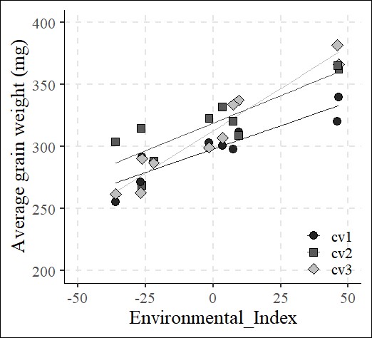
The slope of cv1 is the flattest, while cv3 is the steepest among three genotypes, as indicated by the coefficient_AGW. Therefore, cv1 shows the most stability for grain weight, whereas cv3 is more variable or plastic across environments.
□ code summary: https://github.com/agronomy4future/r_code/blob/main/R_package__fwrmodel.ipynb