[STAT Article] Step-by-Step Guide to Calculating and Analyzing Principal Component Analysis (PCA) by Hand

Principal Component Analysis (PCA) is a statistical technique used for dimensionality reduction while preserving as much variability in the data as possible. It transforms the original variables in a dataset into a new set of uncorrelated variables called principal components, ordered by the amount of variance they capture from the original dataset.
Here’s the step of Principal Component Analysis (PCA).
1. Standardize the Data:
Since PCA is affected by the scale of the variables, it often begins with standardizing the dataset, so each feature contributes equally to the analysis.

2. Compute the Covariance Matrix:
This step captures the relationships between the features. A high covariance between two variables suggests they are strongly related.

3. Calculate Eigenvalues and Eigenvectors:
Eigenvalues represent the amount of variance captured by each principal component, while eigenvectors represent the direction of these components.

4. Sort and Select Principal Components:
The principal components are ranked by the eigenvalues. You select the top components, which capture the majority of the variance, to reduce dimensionality without losing significant information.
When you conduct PCA, do you simply accept the results provided by the software without considering the preceding steps? If we just accept results without any doubts, we never understand the principle of PCA.
In this time, I’ll introduce how PCA is calculated step by step, and if you read this post, I believe you can fully understand the concept of PCA.
Here is one data for corn. Let’s say we measured kernel number per ear (KN), average of kernel weight per ear (KW) and cob dry weight per ear (Cob weight) about five corn genotypes.
| Genotype | KN | KW | Cob weight |
| A | 616 | 335.5 | 242.5 |
| B | 576 | 359.8 | 237.2 |
| C | 615 | 335.6 | 234.3 |
| D | 590 | 357.8 | 243.8 |
| E | 606 | 333.3 | 232.6 |
If you follow step by step, it’s a simple mathematics in middle school.
1. Standardize the Data

Using mean and standard deviation, we can convert each data to Z value.
| Genotype | KN | KW | Cob weight |
| A | 616 | 335.5 | 242.5 |
| B | 576 | 359.8 | 237.2 |
| C | 615 | 335.6 | 234.3 |
| D | 590 | 357.8 | 243.8 |
| E | 606 | 333.3 | 232.6 |
| Mean | 600.6 | 344.4 | 238.1 |
| Stdev | 17.3 | 13.2 | 4.9 |
As an example, I show the formula how 0.90 and -1.11 were calculated in Excel. If you follow this equation z = (x - µ)/σ , simply we can calculate the standardized (or normalized) data.

| Genotype | KN | KW | Cob weight |
| A | 0.89 | -0.67 | 0.90 |
| B | -1.43 | 1.17 | -0.18 |
| C | 0.83 | -0.67 | -0.77 |
| D | -0.61 | 1.02 | 1.16 |
| E | 0.31 | -0.84 | -1.11 |
| Mean | 0 | 0 | 0 |
| Stdev | 1 | 1 | 1 |
For more details, please visit below my posts.
□ Reading Materials
■ [Data article] Why is data normalization necessary when visualizing data?
■ [Data article] Data Normalization Techniques: Excel and R as the Initial Steps in Machine Learning
Recently, I developed an R package called normtools() to easily normalize datasets. I’ll show you how easily we can standardize (or normalize) data.
# to create dataset
group=rep(c("2024"),5)
genotype=c("A","B","C","D","E")
kn=c(616,576,615,590,606)
kw=c(335.5,359.8,335.6,357.8,333.3)
cob_weight=c(242.5,237.2,234.3,243.8,232.6)
df=data.frame(group, genotype,kn,kw,cob_weight)

# to install the package
if(!require(remotes)) install.packages("remotes")
if (!requireNamespace("normtools", quietly = TRUE)) {
  remotes::install_github("agronomy4future/normtools")
}
library(remotes)
library(normtools)

# to run normtools()
z_test= normtools(df, c("group"),c("kn","kw","cob_weight"), method= 1) # 1 or "z_test"
z_test
I added a column named 'group,' which is a dummy variable to enable normalization within groups. If there is only one level, such as 2024, all data will be normalized together. If there are two levels, such as 2023 and 2024, the data will be normalized separately within each level.
If you run the above code, you can obtain the normalized dataset as follows:
  group genotype  kn    kw cob_weight Normalized_kn mean_kn    sd_kn Normalized_kw mean_kw   sd_kw Normalized_cob_weight mean_cob_weight sd_cob_weight
1  2024        A 616 335.5      242.5     0.8923976   600.6 17.25688    -0.6744263   344.4 13.1964             0.8959603          238.08      4.933255
2  2024        B 576 359.8      237.2    -1.4255182   600.6 17.25688     1.1669848   344.4 13.1964            -0.1783812          238.08      4.933255
3  2024        C 615 335.6      234.3     0.8344497   600.6 17.25688    -0.6668485   344.4 13.1964            -0.7662285          238.08      4.933255
4  2024        D 590 357.8      243.8    -0.6142477   600.6 17.25688     1.0154284   344.4 13.1964             1.1594780          238.08      4.933255
5  2024        E 606 333.3      232.6     0.3129186   600.6 17.25688    -0.8411384   344.4 13.1964            -1.1108286          238.08      4.933255
This package provides normalized data along with the mean and standard deviation used for normalization. To simplify, I’ll select only the normalized data.
df1= data.frame(subset(z_test, select=c("Normalized_kn","Normalized_kw","Normalized_cob_weight")))

df1
  Normalized_kn Normalized_kw Normalized_cob_weight
1     0.8923976    -0.6744263             0.8959603
2    -1.4255182     1.1669848            -0.1783812
3     0.8344497    -0.6668485            -0.7662285
4    -0.6142477     1.0154284             1.1594780
5     0.3129186    -0.8411384            -1.1108286
This data matches what I calculated manually. For more details, please visit my post below introducing the package.
■ Practices in Data Normalization using normtools() in R
2. Calculating covariance
Once data normalization is complete, the next step is to calculate the covariance among variables. I calculated the covariance in Excel using the following equation.
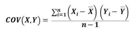

I leave formula in Excel below for clear understanding.
#Excel formula
KN ↔ KN =(((B2-B7)*(B2-B7))+((B3-B7)*(B3-B7))+((B4-B7)*(B4-B7))+((B5-B7)*(B5-B7))+((B6-B7)*(B6-B7)))/(5-1) = 1.00

KN ↔ KW =(((B2-B7)*(C2-C7))+((B3-B7)*(C3-C7))+((B4-B7)*(C4-C7))+((B5-B7)*(C5-C7))+((B6-B7)*(C6-C7)))/(5-1) =-0.93

KN ↔ Cob weight =(((B2-B7)*(D2-D7))+((B3-B7)*(D3-D7))+((B4-B7)*(D4-D7))+((B5-B7)*(D5-D7))+((B6-B7)*(D6-D7)))/(5-1) =-0.17

KW ↔ KN =(((B2-B7)*(C2-C7))+((B3-B7)*(C3-C7))+((B4-B7)*(C4-C7))+((B5-B7)*(C5-C7))+((B6-B7)*(C6-C7)))/(5-1) =-0.93

KW ↔ KW =(((C2-C7)*(C2-C7))+((C3-C7)*(C3-C7))+((C4-C7)*(C4-C7))+((C5-C7)*(C5-B7))+((C6-B7)*(C6-C7)))/(5-1) = 1.00

KW ↔ Cob weight =(((C2-C7)*(D2-D7))+((C3-C7)*(D3-D7))+((C4-C7)*(D4-D7))+((C5-C7)*(D5-D7))+((C6-C7)*(D6-D7)))/(5-1) =0.45

Cob weight ↔ KN =(((B2-B7)*(D2-D7))+((B3-B7)*(D3-D7))+((B4-B7)*(D4-D7))+((B5-B7)*(D5-D7))+((B6-B7)*(D6-D7)))/(5-1) =-0.17

Cob weight ↔ KW =(((C2-C7)*(D2-D7))+((C3-C7)*(D3-D7))+((C4-C7)*(D4-D7))+((C5-C7)*(D5-D7))+((C6-C7)*(D6-D7)))/(5-1) =0.45

Cob weight ↔ Cob weight =(((D2-D7)*(D2-D7))+((D3-D7)*(D3-D7))+((D4-D7)*(D4-D7))+((D5-D7)*(D5-D7))+((D6-D7)*(D6-D7)))/(5-1) = 1.00
However, is that really necessary to calculate covariance like this? If you fully understand covariance, you’re familiar with below equation I suggest.
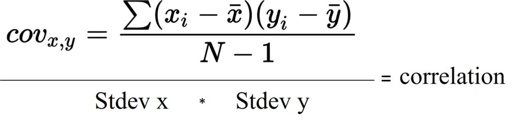
If we divide covariance by multiplication of standard deviation of x and y, it will be correlation (r). That is, the below correlation formula we usually know is the same as what I suggested above.
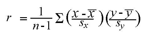
Let’s think about this. We already normalized data, which means standard deviation is 1. Then, the below equation would be possible as standard deviation of x and y is 1.
cov (x,y) = r
For more details, please visit below my post and YouTube video.
□ Reading Materials
□ Simple linear regression (1/5)- correlation and covariance
It means when data is normalized, covariance and correlation will be the same. In Excel, we can easily obtain correlation.


If you follow above steps, you can obtain correlation like below.

Let’s copy and paste each value in the same relationship to the blank cells, and this result will be the same as what we calculated by hand.

In R, we can easily obtain correlation.
cor(df1)
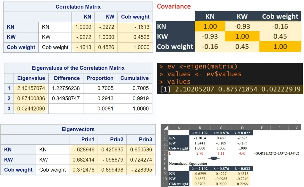
Normalized_kn Normalized_kw Normalized_cob_weight
Normalized_kn 1.0000000 -0.9271996 -0.1613366
Normalized_kw -0.9271996 1.0000000 0.4525646
Normalized_cob_weight -0.1613366 0.4525646 1.0000000Or, in R, we can also obtain covariance.
cov(df1)
                      Normalized_kn Normalized_kw Normalized_cob_weight
Normalized_kn             1.0000000    -0.9271996            -0.1613366
Normalized_kw            -0.9271996     1.0000000             0.4525646
Normalized_cob_weight    -0.1613366     0.4525646             1.0000000
Either way, the value is the same. This is because the data is normalized, and the standard deviation is 1. Therefore, in normalized data, covariance and correlation will be the same. Anyway, this data matches what I calculated in Excel.
3. Eigenvector and Eigenvalue
From here, we need to understand the concept of vector. However, it would not be necessary to fully understand what it is. Instead, let’s grab the concept we need to analyze PCA.
Eigenvalue is called lamda (λ), and here is a formula
Ax=λx
and this formula is also explained as below
(A−λI)x=0

For example, with A matrix and λI matrix, we can think the right matrix. Then, the covariance table we calculated will be expressed as below.

This is 3×3 matrix. Unlike 2×2 matrix, 3×3 matrix will be calculated as below

First, let’s calculate eigenvalue, λ

{(1-λ){(1-λ)(1-λ)-(0.450.45)} - {-0.93((-0.93(1-λ))-(0.45-0.16))} + {-0.16((-0.930.45)-((1-λ)*-0.16))} = 0
Now we need to find λ. We might be able to primitively calculate in our notes, but let’s work smart!! Using a simple R code, we can easily obtain λ.
matrix= matrix(c(1, -0.93, -0.16, -0.93, 1, 0.45, -0.16, 0.45, 1), 3, 3, byrow=TRUE)

matrix
      [,1]  [,2]  [,3]
[1,]  1.00 -0.93 -0.16
[2,] -0.93  1.00  0.45
[3,] -0.16  0.45  1.00
Now I generated covariance table as 3×3 matrix. Then, I use the below R code.
ev= eigen(matrix)
values= ev$values

values
[1] 2.10205207 0.87571854 0.02222939
Now eigenvalue was calculated.
λ = 2.10205207, 0.87571854, 0.02222939
To verify this value is correct, I’ll substitute those λ values in (1-λ){(1-λ)(1-λ)-(0.450.45)} - {-0.93((-0.93(1-λ))-(0.45-0.16))} + {-0.16((-0.930.45)-((1-λ)*-0.16))} = 0

When we substitute each λ value in the equation, all of them becomes 0.
Now we can obtain eigenvector.
(example)
λ = ≈ 2.102

When λ is ≈ 2.102, this is how to calculate eigenvector.
-1.11 x1 -0.93 x2 – 0.17 x3 = 0 —— (a)
-0.93 x1 -1.11 x2 + 0.45 x3 = 0 —— (b)
-0.17 x1 +0.45 x2 – 1.11 x3 = 0 —— (c)
Now we need to find x1, x2, x3. Again!! we might be able to primitively calculate in our notes, but there are many websites to calculate eigenvector.
For example, I’ll obtain eigenvector in below website.
https://www.symbolab.com/solver/matrix-eigenvectors-calculator

First, let’s generate 3×3 matrix, and input covariance values, and in front of the matrix, type ‘Eigenvalue’

The website shows the λ equation
{(1-λ){(1-λ)(1-λ)-(0.450.45)} - {-0.93((-0.93(1-λ))-(0.45-0.16))} + {-0.16((-0.930.45)-((1-λ)*-0.16))} = 0
is summarized as
-λ3 + 3λ2 - 1.907λ + 0.04092 = 0
and λ is ≈ 0.022, ≈ 0.876, ≈2.102, which is the same value we obtained from R. Now we can trust eigenvalues R provides.
Now, let’s calculate eigenvectors when λ is ≈2.102. Again!! let’s generate 3×3 matrix, and input covariance values, but now in front of the matrix, type ‘Eigenvectors’

Eigenvectors corresponding to each Eigenvalue was calculated. When λ is ≈2.102, eigenvectors are ≈ – 1.701 , 1.844, 1
Let’s check this values are correct in Excel. If those values are correct, in below equation, when we input x1 ≈ – 1.701, x2 ≈ 1.844 , x3 ≈ 1, all equation will be 0.
-1.11 x1 -0.93 x2 – 0.17 x3 = 0 —— (a)
-0.93 x1 -1.11 x2 + 0.45 x3 = 0 —— (b)
-0.17 x1 +0.45 x2 – 1.11 x3 = 0 —— (c)

All equations become 0, and therefore when λ is ≈2.102 the below matrix is validated.

If we check eigenvectors from the other two λ values, the matrix is also validated.
4. Calculating component score
Now, let’s sort eigenvalue from large to small values (2.102, 00876, 0.022).

To verify these values are correct, I’ll check in R.
ev= eigen(matrix)

ev
eigen() decomposition
$values
[1] 2.10205207 0.87571854 0.02222939

$vectors
           [,1]        [,2]       [,3]
[1,]  0.6299076  0.42274681 -0.6515379
[2,] -0.6827452 -0.09849582 -0.7239873
[3,] -0.3702371  0.90087941  0.2265851
Eigenvectors are different from what we calculated. How these values were calculated in R?
In R, eigenvectors are ‘Normalized Eigenvector.’ The way to normalize eigenvectors is like below. Simply, it’s kind of reducing the length of vector.

Based on the above equation, I re-calculated eigenvectors. For your understanding, I leave a formula about how 4.41 was calculated in Excel.

Now our eigenvectors are the same as R provided. The difference of positive and negative values will be explained in the last part.
Using these eigenvectors, we can calculate component score per genotype.
Do you remember we normalized our data in the first step? Now we use the normalized data to calculate component score.

For example, component score of Genotype A will be calculated as
Genotype APC1 = -0.6299*KN + 0.6827*KW + 0.3702*Cob weightPC2 = 0.4227*KN + -0.0985*KW + 0.9009*Cob weightPC3 =-0.6515*KN + -0.7240*KW + 0.2266*Cob weight
In Genotype A, KN = 0.89, KW = -0.67, Cob weight = 0.90.
Therefore, it will be calculated as below
PC1 = -0.6299*0.89 + 0.6827*-0.67 + 0.3702*0.90 = -0.6848PC2 = 0.4227*0.89 + -0.0985*-0.67+ 0.9009*0.90 = 1.253PC3 = -0.6515*0.89 + -0.7240*-0.67 + 0.2266*0.90 = 1.109
There are many websites to calculate matrix. In this website, let’s generate 5×3 matrix and 3×3 matrix, and input the values (https://matrix.reshish.com/multiplication.php)

and the result will be

It was a long journey!!! Here is the final component score!!

■ Principal Components Analysis using R
We primitively calculated PCA by hand. Now let’s verify this calculation is correct. I’ll calculate each process I introduced using R.
1. to create data
First, I’ll create the dataset.
genotype=c("A","B","C","D","E")
kn=c(616,576,615,590,606)
kw=c(335.5,359.8,335.6,357.8,333.3)
cob_weight=c(242.5,237.2,234.3,243.8,232.6)
df=data.frame(genotype,kn,kw,cob_weight)

df
  genotype  kn    kw    cob_weight
1        A  616  335.5  242.5
2        B  576  359.8  237.2
3        C  615  335.6  234.3
4        D  590  357.8  243.8
5        E  606  333.3  232.6
However, to conduct PCA, categorical variable should be row name. So, I’ll change ‘genotype’ as the row name.
genotype=c("A","B","C","D","E")
kn=c(616,576,615,590,606)
kw=c(335.5,359.8,335.6,357.8,333.3)
cob_weight=c(242.5,237.2,234.3,243.8,232.6)
df=data.frame(kn,kw,cob_weight)
row.names(df)= genotype

df
   kn    kw cob_weight
A 616 335.5      242.5
B 576 359.8      237.2
C 615 335.6      234.3
D 590 357.8      243.8
E 606 333.3      232.6
2. to normalize data
I’ll normalize data using scale()
df$kn= scale(df$kn, center=TRUE, scale=TRUE)
df$kw= scale(df$kw, center=TRUE, scale=TRUE)
df$cob_weight= scale(df$cob_weight, center=TRUE, scale=TRUE)

df
          kn         kw cob_weight
A  0.8923976 -0.6744263  0.8959603
B -1.4255182  1.1669848 -0.1783812
C  0.8344497 -0.6668485 -0.7662285
D -0.6142477  1.0154284  1.1594780
E  0.3129186 -0.8411384 -1.1108286
3. Calculating covariance
In R, it’s not necessary to do this process when conducting PCA, but to verify our calculation is correct, let’s check the covariance in R.
cor(df)
                   kn         kw cob_weight
kn          1.0000000 -0.9271996 -0.1613366
kw         -0.9271996  1.0000000  0.4525646
cob_weight -0.1613366  0.4525646  1.0000000
3. Eigenvector
Now, it’s the time to obtain eigenvectors
pca= prcomp(df)

> pca
Standard deviations (1, .., p=3):
[1] 1.4496795 0.9348841 0.1562719

Rotation (n x k) = (3 x 3):
                  PC1         PC2        PC3
kn         -0.6289457 -0.42563473 -0.6505862
kw          0.6824142  0.09867947 -0.7242743
cob_weight  0.3724758 -0.89949844  0.2283952
In R, eigenvectors are quickly calculated. It’s the same as what we calculated by hand. The difference of positive and negative values will be explained in the last part.
We can skip the step ‘2. Normalize data’ by directly adding scale=TRUE inside prcomp().”
genotype=c("A","B","C","D","E")
kn=c(616,576,615,590,606)
kw=c(335.5,359.8,335.6,357.8,333.3)
cob_weight=c(242.5,237.2,234.3,243.8,232.6)
df=data.frame(kn,kw,cob_weight)
row.names(df)= genotype

pca= prcomp(df, scale=TRUE)

pca
Standard deviations (1, .., p=3):
[1] 1.4496795 0.9348841 0.1562719

Rotation (n x k) = (3 x 3):
                  PC1         PC2        PC3
kn         -0.6289457 -0.42563473 -0.6505862
kw          0.6824142  0.09867947 -0.7242743
cob_weight  0.3724758 -0.89949844  0.2283952
Calculating eigenvectors by hand was a complex process, but in R, we can obtain them in just 5 seconds. However, now we understand how eigenvectors are calculated, meaning we know the underlying principles.
4. Calculating component score
Now, let’s calculate component score. We calculated component score as multiplying the matrix between normalized data and eigenvectors, and the same code is below.
round(scale(df) %*% pca$rotation,3)
or
round(pca$x,3)

     PC1    PC2    PC3
A -0.688 -1.252  0.113
B  1.626  0.882  0.041
C -1.265  0.268 -0.235
D  1.511 -0.681 -0.071
E -1.185  0.783  0.152
The result is the same as what we calculated by hand. The difference in positive and negative values will be explained in the final section. The small discrepancy is due to rounding at different decimal points.
■ Making a graph
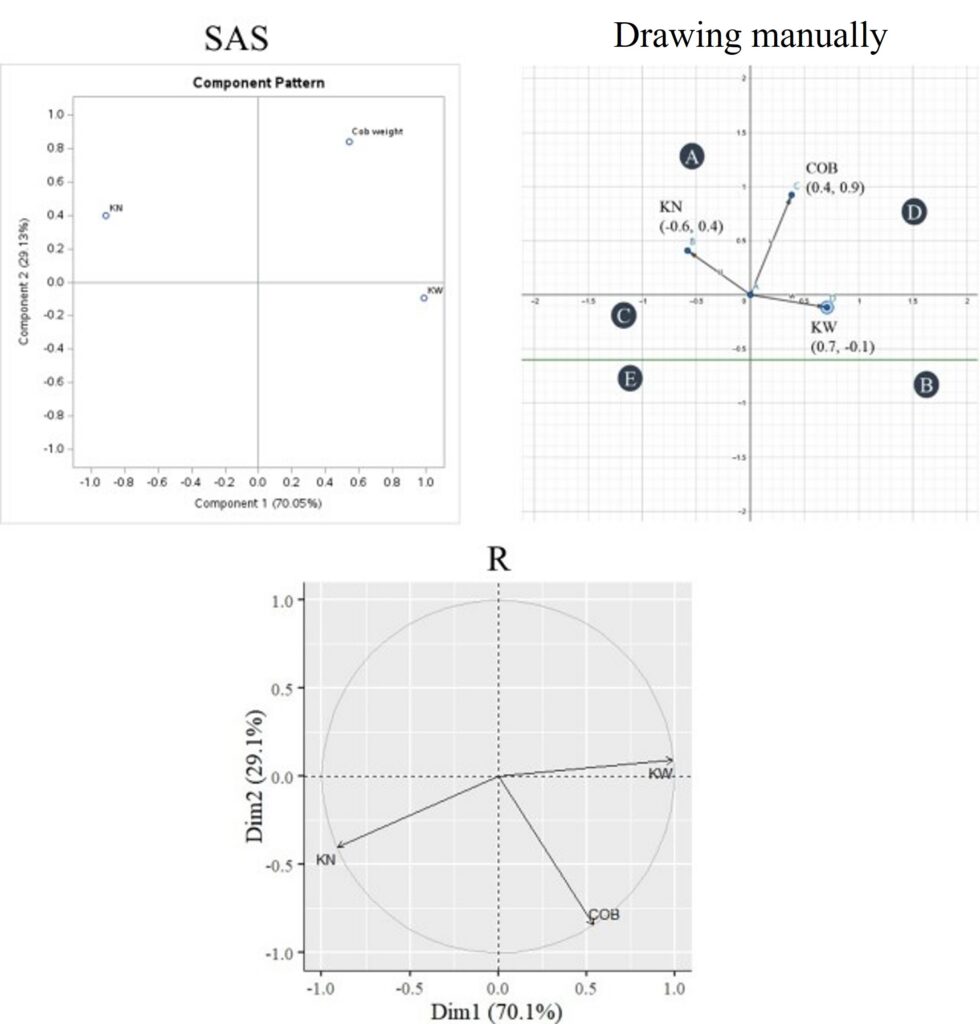
In this website (https://www.geogebra.org/calculator), let’s draw a graph about eigenvectors and component scores. I compared the value of eigenvectors and component scores from R (left graph) with the values from my calculation (right graph).
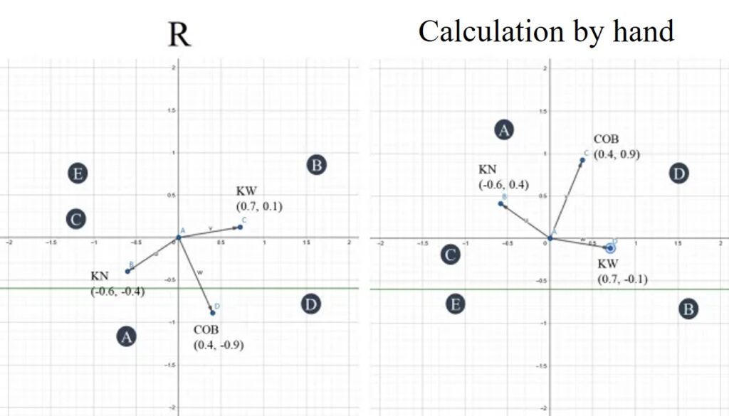
The difference in positive and negative values between R and my calculation is shown in the graph above. If we flip the left graph, it will match the right graph. Nonetheless, the interpretation of the results for both graphs remains the same.
I’ll draw a graph using R.
if (require("factoextra")== F) install.packages("factoextra")
library(factoextra)

fviz_pca_var(pca, labelsize= 4, repel= TRUE) +
  labs(title="") +
  theme_grey(base_size=18, base_family="serif")+
  theme(axis.line= element_line(size=0.5, colour="black"),
        axis.title.y= element_text (margin = margin(t=0, r=0, b=0, l=0)),
        plot.margin= margin(-0.7,-0.7,0,-0.7,"cm")) +
  windows(width=5.5, height=5)
It’s the same as what I drew by hand.
If you copy and paste the below code in R, you can obtain the same graph above.
if (require("factoextra")== F) install.packages("factoextra")
library(factoextra)

genotype=c("A","B","C","D","E")
kn=c(616,576,615,590,606)
kw=c(335.5,359.8,335.6,357.8,333.3)
cob_weight=c(242.5,237.2,234.3,243.8,232.6)
df=data.frame(kn,kw,cob_weight)
row.names(df)= genotype

pca= prcomp(df, scale=TRUE)

fviz_pca_var(pca, labelsize=4, repel=TRUE) +
  labs(title="") +
  theme_grey(base_size=18, base_family="serif")+
  theme(axis.line=element_line(size=0.5, colour="black"),
        axis.title.y=element_text(margin=margin(t=0,r=0,b=0,l=0)),
        plot.margin=margin(-0.7,-0.7,0,-0.7,"cm")) +
windows(width=5.5, height=5)
■ How to interpret the graph?
1) The range of eigenvector
The eigenvector is normalized, with values always ranging between -1 and 0. If you observe a different data range in PC1 and PC2, it suggests that those eigenvectors were not normalized. When performing PCA, the eigenvectors are typically normalized by default.
2) Variance of components
summary(pca)

Importance of components:
                          PC1    PC2     PC3
Standard deviation     1.4497 0.9349 0.15627
Proportion of Variance 0.7005 0.2913 0.00814
Cumulative Proportion  0.7005 0.9919 1.00000
This is the summary of component scores. It shows standard deviation, and cumulative variance in PC1 to PC3. It says PC1 and PC2 account for 99% variance from the whole data.
In standard deviation, let’s check variance as squaring (s =√v, v = s2)
1.44972 = 2.10
0.93492 = 0.87
0.156272 = 0.02
Do you remember those values? We encountered them when we calculated PCA step-by-step—they’re the eigenvalues.

That is, eigenvalue (λ) is variance of components. That’s why we sort from the large value.
In PC1, it accounts for 70.1% of the total variance, and in PC2, it accounts for 29.1% of the total variance. How were these values calculated?
Let’s add up all eigenvalue (λ)
2.102 + 0.876 + 0.022 ≈ 3
and
2.102 / 3 ≈ 0.70 (variance ratio in PC1)
0.876 / 3 ≈ 0.29 (variance ratio inPC2)
3) Interpretation of vector
A) Direction and proximity of vector

A and B is negatively correlated (in PC1, A is positive value, while B is negative value).
A and C is positively correlated (in PC1, both A and B are positive value).
If two vectors are adjacent, and the angle between two vectors is small, two variables are positively correlated. If the angle between two vectors is 90°, two variables are independent.
B) Length of vector

As mentioned above, A and B; and C and D are negatively correlated, but A and B highly affects variance of the data while C and D less affect the variance. It means A and B is the most important variables to explain the whole data.
Tip!! PCA analysis using SAS Studio
| Genotype | KN | KW | Cob weight |
| A | 616 | 335.5 | 242.5 |
| B | 576 | 359.8 | 237.2 |
| C | 615 | 335.6 | 234.3 |
| D | 590 | 357.8 | 243.8 |
| E | 606 | 333.3 | 232.6 |

In SAS STUDIO, please go to Tasks and Utilities and select Multivariate Analysis > Principle Component Analysis. Then choose KN, KW, Cob weight at Analysis variables in ROLES section.
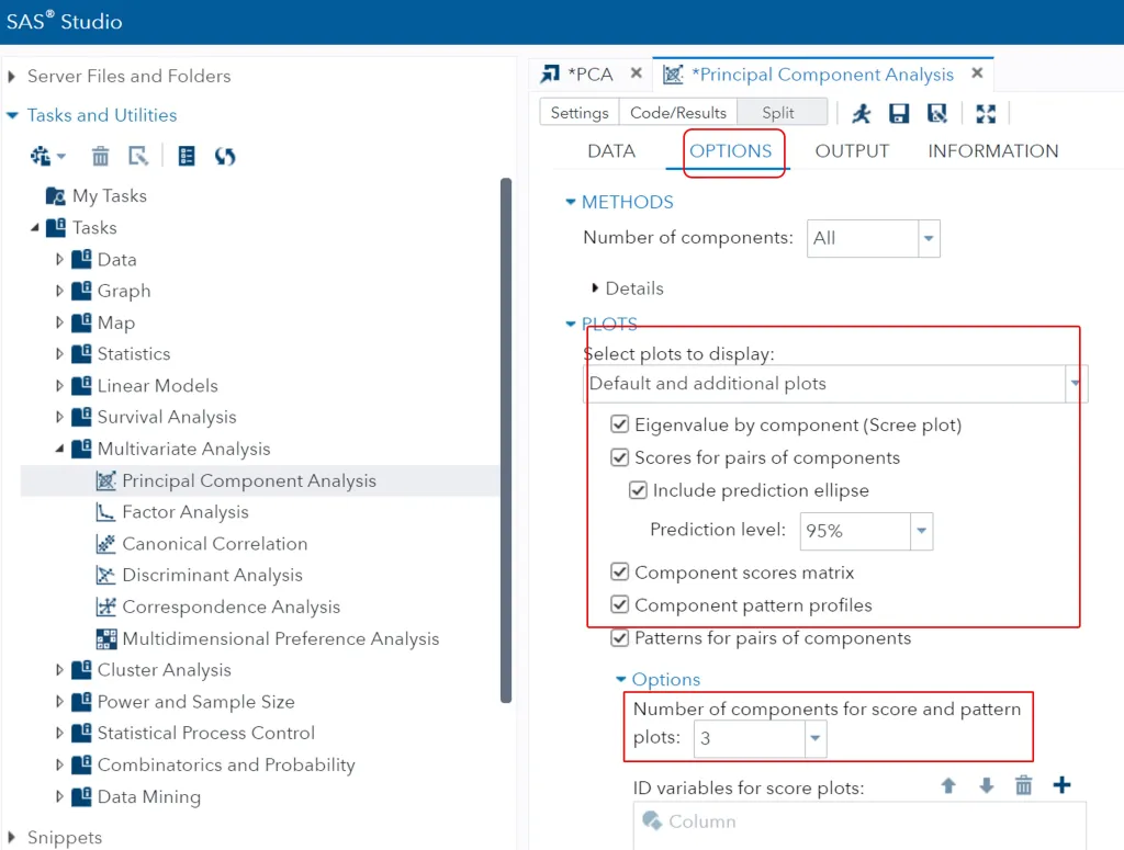
I’d like to see the outcome from PC1, PC2, PC3, and therefore I selected 3 in Number of components for score and pattern. Then, in Select plots to display, please select Default and additional plots and click all options. Then click the run button.
Let’s compare the outcomes provided by SAS with those we calculated by hand. All values match. From now on, we can fully understand the values that statistical programs provide for PCA analysis and have gained insight into the underlying principles.
Now, let’s compare the graphs. When we compared the graphs, we drew manually with those provided by R, we noticed they were inverted vertically. However, when we compared the manually drawn graphs with those from SAS, they were identical. Therefore, the inversion of the graph doesn’t affect the interpretation, as the pattern remains consistent.
We aim to develop open-source code for agronomy (kimjk@agronomy4future.com)
© 2022 – 2025 https://agronomy4future.com – All Rights Reserved.
Last Updated: 02/18/2025