[R package] Probability Distribution and Z-Score Calculation Function (feat. probdistz)
■ Introduction
■ What is Probability Density Function (PDF) and Cumulative Distribution Function (CDF): How to calculate using Excel and R?
In my previous post, I explained what the Probability Density Function (PDF) and the Cumulative Distribution Function (CDF) are. I also explained the formula for the PDF and demonstrated how to manually calculate it in Excel.
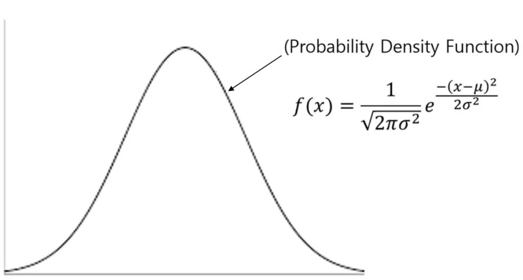

Additionally, I mentioned the Excel function that performs the same calculation for the PDF, as follows:
=NORM.DIST(x, mean, stdev, FALSE) I then introduced how to create a probability distribution graph in R using stat_function(). To use stat_function(), you need to specify the mean and standard deviation of your data in the code. For example, this is an example of the stat_function().
ggplot(data=df, aes(x=yield)) +
   stat_function(data=df ,aes(x=yield),color="blue",size=1,
     fun=dnorm, args=c(mean=mean(df$yield), sd=sd(df$yield))) +
I initially thought I could create a probability distribution graph using a simple code like geom_line() instead of stat_function(), which requires typing in the mean and standard deviation. Therefore, recently, I developed an R package called probdistz() to facilitate this process.
□ Github: https://github.com/agronomy4future/probdistz/blob/main/README.md
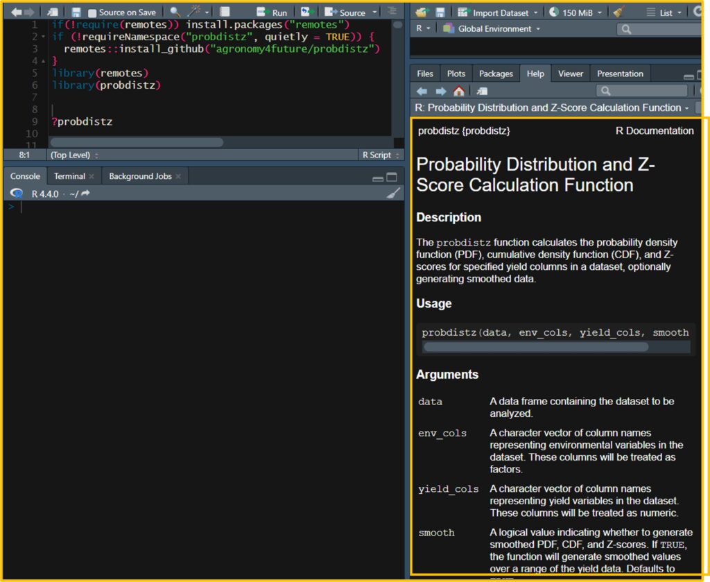
■ Package installation
First, let’s install the package.
if(!require(remotes)) install.packages("remotes")
if (!requireNamespace("probdistz", quietly = TRUE)) {
  remotes::install_github("agronomy4future/probdistz")
}
library(remotes)
library(probdistz)
If you type ?probdistz in your R script, you can view detailed information about this package.
■ Code format
The basic format of the code is as follows:
probdistz(data, env_cols, yield_cols, smooth= TRUE)
*smooth= TRUE or FALSE (Default is TRUE)

□ data refers to the dataset you want to analyze.
□ env_cols specifies the grouping for calculating the PDF and CDF. For example, if you set env_cols= c("field", "genotype"), the PDF and CDF will be calculated per genotype within each field. Conversely, if you set env_cols= c("genotype"), the PDF and CDF will be calculated per genotype across all environments.
□ yield_cols specifies the independent variables for which you want to calculate the PDF and CDF.
When selecting smooth= TRUE, the probdistz() package predicts additional data to compensate for a lack of sample size, based on 6σ, and uses this to calculate the PDF, CDF, and Z-score, resulting in a continuous probability curve. On the contrary, when selecting smooth= FALSE, the probdistz() package calculates the PDF, CDF, and Z-score based on the actual dataset. Therefore, if the datapoints are limited, the probability curve may not be connected.
■ Upload the data for practice
Let’s practice using this code with an actual dataset. Please copy and paste the code below into your R script.
if(!require(readr)) install.packages("readr")
library(readr)
github="https://raw.githubusercontent.com/agronomy4future/raw_data_practice/main/grains.csv"
df = data.frame(read_csv(url(github), show_col_types=FALSE))
and you can obtain the below dataset. This data is grain number per certain unit and grain weight (mg) data across different environmental conditions.
head(df,5)
     field genotype block        stage   treatment shoot      grain_number grain_weight
1 up_state     cv_1     I pre_anthesis treatment_1 main stem  513          49.26
2 up_state     cv_1     I pre_anthesis treatment_1 tillers    268          44.68
3 up_state     cv_2     I pre_anthesis treatment_1 main stem  616          45.19
4 up_state     cv_2     I pre_anthesis treatment_1 tillers    83           44.34
5 up_state     cv_1     I pre_anthesis     control main stem  516          48.25
.
.
.
First, let’s create a Probability Density Function (PDF) curve using stat_function(). Before doing that, you need to decide within which groups you’ll calculate the PDF.
The dataset is structured as follows:
| Independent variable | Number of levels | Remarks |
| Field | 2 | Up state, Down state |
| Genotype | 3 | CV1, CV2, CV3 |
| Block | 3 | I, II, III |
| Stage | 2 | pre_anthesis ,post_anthesis |
| Treatment | 3 | Control, treatment 1, treatment 2 |
| Shoot | 2 | Main stem, tillers |
| Dependent variable | ||
| Gran number | ||
| Grain weight |
First, I want to visualize the probability distribution of grain weight per genotype across all environments.
ggplot(data=df, aes(x=grain_weight)) +

  stat_function(data=subset(df, genotype=="cv_1"), aes(color= "cv_1"), linewidth=1,
    fun=dnorm, args=list(mean=mean(subset(df, genotype=="cv_1")$grain_weight, na.rm=TRUE),
    sd=sd(subset(df, genotype=="cv_1")$grain_weight, na.rm=TRUE))) +

  stat_function(data=subset(df, genotype=="cv_2"), aes(color= "cv_2"), linewidth=1,
    fun=dnorm, args=list(mean=mean(subset(df, genotype=="cv_2")$grain_weight, na.rm=TRUE),
    sd=sd(subset(df, genotype=="cv_2")$grain_weight, na.rm=TRUE))) +

  stat_function(data=subset(df, genotype=="cv_3"), aes(color= "cv_3"), linewidth=1,
    fun=dnorm, args=list(mean=mean(subset(df, genotype=="cv_3")$grain_weight, na.rm=TRUE),
    sd=sd(subset(df, genotype=="cv_3")$grain_weight, na.rm=TRUE))) +

scale_color_manual(name= "Genotype", values = c("cv_1"="black", "cv_2"="red", "cv_3"="blue")) +
scale_x_continuous(breaks=seq(0,80,20), limits=c(0,80)) +
scale_y_continuous(breaks=seq(0,0.15,0.03), limits=c(0,0.15)) +
labs(x="Wheat grain weight (mg)", y="Frequency") +
theme_classic(base_size=15, base_family="serif") +
theme(legend.position=c(0.85, 0.85),
      legend.title=element_blank(),
      legend.key=element_rect(color="white", fill="white"),
      legend.text=element_text(family="serif", face="plain", size=15, color= "Black"),
      legend.background=element_rect(fill="white"),
      axis.line=element_line(linewidth=0.5, colour="black"))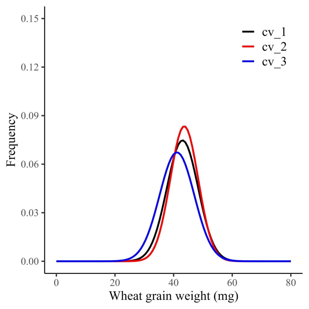
This is the probability distribution of grain weight across all environments.
Next, I want to create a Probability Density Function (PDF) curve for each genotype, categorized by fields. The df dataset contains data from two fields: upstate and downstate. I want to analyze the distribution for either of these locations.
For example, I’ll slightly modify the previous code to generate a PDF curve for each genotype in the upstate field.
ggplot(data=subset(df, field=="up_state"), aes(x=grain_weight)) +

 stat_function(data=subset(subset(df, field=="up_state"), genotype=="cv_1"),
  aes(color="cv_1"), linewidth=1, fun=dnorm,
  args=list(mean=mean(subset(subset(df, field=="up_state"), genotype=="cv_1")$grain_weight, na.rm=TRUE),
  sd=sd(subset(subset(df, field=="up_state"), genotype=="cv_1")$grain_weight, na.rm=TRUE))) +

 stat_function(data=subset(subset(df, field=="up_state"), genotype=="cv_2"),
  aes(color="cv_2"), linewidth=1, fun=dnorm,
  args=list(mean=mean(subset(subset(df, field=="up_state"), genotype=="cv_2")$grain_weight, na.rm=TRUE),
  sd=sd(subset(subset(df, field=="up_state"), genotype=="cv_2")$grain_weight, na.rm=TRUE))) +

 stat_function(data=subset(subset(df, field=="up_state"), genotype=="cv_3"),
  aes(color="cv_3"), linewidth=1, fun=dnorm,
  args=list(mean=mean(subset(subset(df, field=="up_state"), genotype=="cv_3")$grain_weight, na.rm=TRUE),
  sd=sd(subset(subset(df, field=="up_state"), genotype=="cv_3")$grain_weight, na.rm=TRUE))) +

 scale_color_manual(name= "Genotype", values = c("cv_1"="black", "cv_2"="red", "cv_3"="blue")) +
 scale_x_continuous(breaks=seq(0,80,20), limits=c(0,80)) +
 scale_y_continuous(breaks=seq(0,0.15,0.03), limits=c(0,0.15)) +
 labs(x="Wheat grain weight (mg)", y="Frequency") +
 theme_classic(base_size=15, base_family="serif") +
 theme(legend.position=c(0.85, 0.85),
       legend.title=element_blank(),
       legend.key=element_rect(color="white", fill="white"),
       legend.text=element_text(family="serif", face="plain", size=15, color= "Black"),
       legend.background=element_rect(fill="white"),
       axis.line=element_line(linewidth=0.5, colour="black"))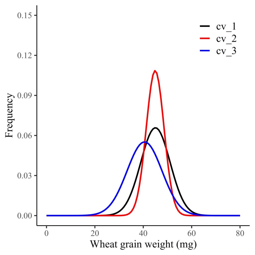
Now, the probability distribution of grain weight per genotype is for upstate field only.
If you change the code to subset(df, field=="down_state") in the code above, you can also generate the graph for the downstate field only.
■ probdistz code for PDF
I developed the probdistz() package. As mentioned above, the basic format of the code is below.
probdistz(data, env_cols, yield_cols, smooth= TRUE)
*smooth= TRUE or FALSE, Default is TRUE
Again, I want to create a Probability Density Function (PDF) curve for each genotype, categorized by field.
head(df,5)
     field genotype block        stage   treatment shoot      grain_number grain_weight
1 up_state     cv_1     I pre_anthesis treatment_1 main stem  513          49.26
2 up_state     cv_1     I pre_anthesis treatment_1 tillers    268          44.68
3 up_state     cv_2     I pre_anthesis treatment_1 main stem  616          45.19
4 up_state     cv_2     I pre_anthesis treatment_1 tillers    83           44.34
5 up_state     cv_1     I pre_anthesis     control main stem  516          48.25
.
.
.
I’ll run code.
# to install package
if(!require(remotes)) install.packages("remotes")
if (!requireNamespace("probdistz", quietly = TRUE)) {
  remotes::install_github("agronomy4future/probdistz")
}
library(remotes)
library(probdistz)
# to run prodistz package
dataA= probdistz(df, env_cols= c("field","genotype"), yield_cols="grain_weight), smooth= TRUE)The output was generated and named dataA, as shown below.
set.seed(100)
dataA[sample(nrow(dataA),5),]
     grain_weight   smooth_pdf   smooth_cdf    smooth_z      field genotype
3786     53.69313 3.036760e-04 9.996976e-01  3.42942943 down_state     cv_1
503      45.21273 6.573905e-02 5.119784e-01  0.03003003   up_state     cv_1
3430     38.00036 7.595374e-02 1.985402e-01 -0.84684685 down_state     cv_1
3696     49.72585 6.898674e-03 9.905716e-01  2.34834835 down_state     cv_1
4090     21.05160 4.985506e-07 4.091933e-07 -4.93093093 down_state     cv_3
.
.
.
You can see the Probability Density Function (PDF), the Cumulative Distribution Function (CDF) and Z-score were generated.
probdistz() package generates additional data based on the mean and standard deviation of the current dataset. This is necessary because, with limited datapoints, a complete probability density curve is not feasible. You may encounter such a difficulty when attempting to create the probability density curve using Excel like below graph.
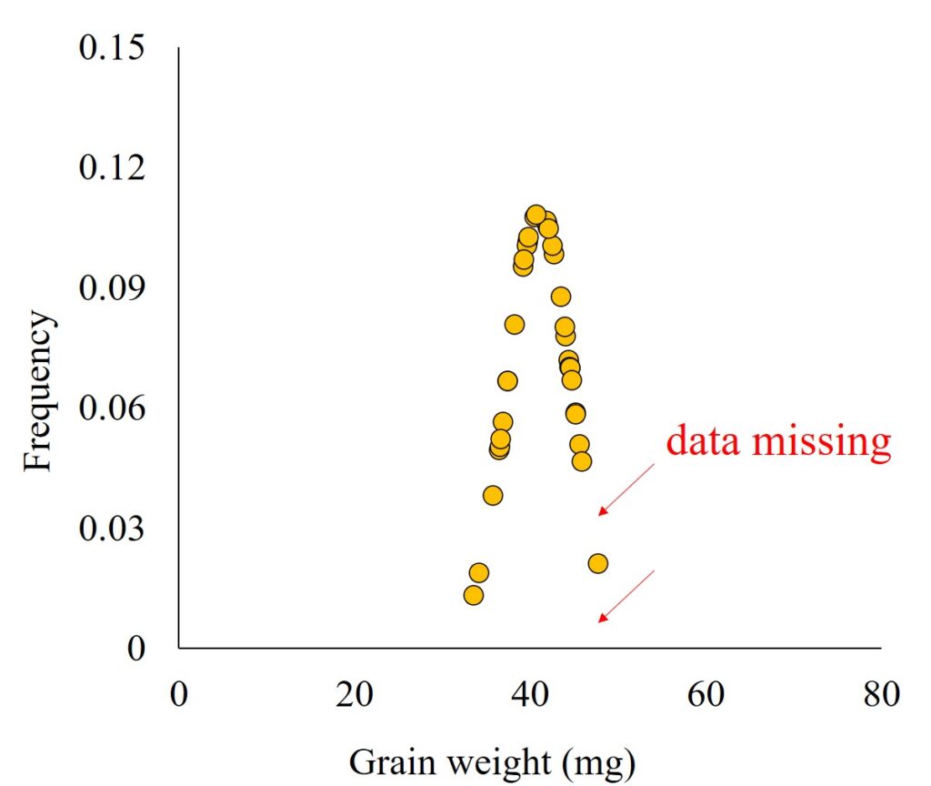
probdistz() package predicts additional data to make up for the missing data based on 6σ.
I’ll filter field, only “up_state” and create the PDF curve.
ggplot(data=subset(dataA, field=="up_state"), aes(x=grain_weight, y=smooth_pdf, color=genotype)) +
  geom_line ()+
  scale_color_manual(name= "Genotype", values= c("cv_1"="black", "cv_2"="red", "cv_3"="blue")) +
  scale_x_continuous(breaks=seq(0,80,20), limits=c(0,80)) +
  scale_y_continuous(breaks=seq(0,0.15,0.03), limits=c(0,0.15)) +
  labs(x="Wheat grain weight (mg)", y="Frequency") +
  theme_classic(base_size=15, base_family="serif") +
  theme(legend.position=c(0.85, 0.85),
        legend.title=element_blank(),
        legend.key=element_rect(color="white", fill="white"),
        legend.text=element_text(family="serif", face="plain", size=15, color= "Black"),
        legend.background=element_rect(fill="white"),
        axis.line=element_line(linewidth=0.5, colour="black"))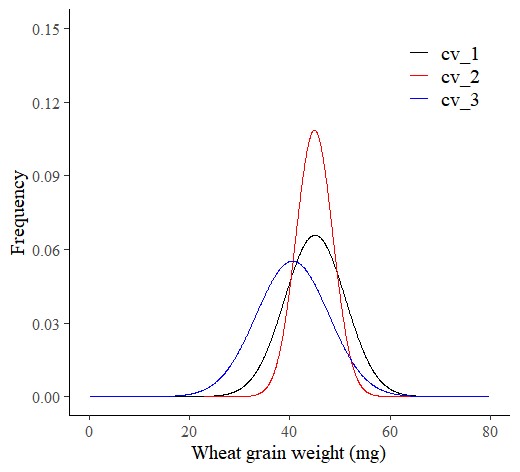
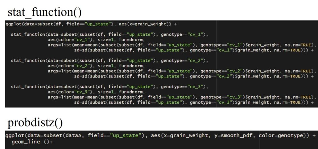
This graph is identical to the one produced using stat_function().
Let’s compare the two codes: stat_function() and probdistz(). The code using probdistz() is much simpler.
Let’s practice the package code more. In this time, I want to create a Probability Density Function (PDF) curve for each genotype ‘across all environments‘.
dataB= probdistz(df, env_cols= c("genotype"), yield_cols="grain_weight", smooth= TRUE)and I’ll create PDF curve.
ggplot(data=dataB, aes(x=grain_weight, y=smooth_pdf, color=genotype)) +
  geom_line ()+
  scale_color_manual(name= "Genotype", values= c("cv_1"="black", "cv_2"="red", "cv_3"="blue")) +
  scale_x_continuous(breaks=seq(0,80,20), limits=c(0,80)) +
  scale_y_continuous(breaks=seq(0,0.15,0.03), limits=c(0,0.15)) +
  labs(x="Wheat grain weight (mg)", y="Frequency") +
  theme_classic(base_size=15, base_family="serif") +
  theme(legend.position=c(0.85, 0.85),
        legend.title=element_blank(),
        legend.key=element_rect(color="white", fill="white"),
        legend.text=element_text(family="serif", face="plain", size=15, color= "Black"),
        legend.background=element_rect(fill="white"),
        axis.line=element_line(linewidth=0.5, colour="black"))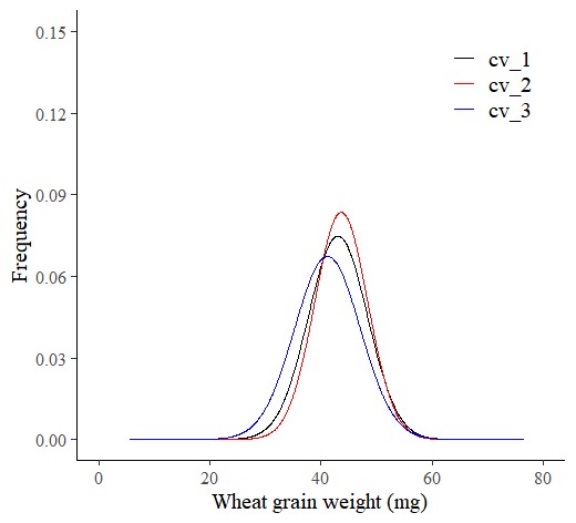
This graph is identical to the one produced using stat_function().
■ probdistz code for CDF
I’ll create the Cumulative Distribution Function (CDF) curve for each genotype, categorized by field. First, I’ll use stat_function() to create the CDF curve for the upstate region only.
head(df,5)
     field genotype block        stage   treatment     shoot grain_number grain_weight
1 up_state     cv_1     I pre_anthesis treatment_1 main stem          513        49.26
2 up_state     cv_1     I pre_anthesis treatment_1   tillers          268        44.68
3 up_state     cv_2     I pre_anthesis treatment_1 main stem          616        45.19
4 up_state     cv_2     I pre_anthesis treatment_1   tillers           83        44.34
5 up_state     cv_1     I pre_anthesis     control main stem          516        48.25

###
ggplot(data=df) +

  stat_function(fun= pnorm,
      args= list(mean= mean(subset(subset(df, field=="up_state"),
      genotype== "cv_1")$grain_weight, na.rm= TRUE),
      sd= sd(subset(subset(df, field=="up_state"), genotype== "cv_1")$grain_weight,
      na.rm= TRUE)), aes(color= "cv_1"), size = 1) +

  stat_function(fun= pnorm,
      args= list(mean= mean(subset(subset(df, field=="up_state"),
      genotype== "cv_2")$grain_weight, na.rm= TRUE),
      sd= sd(subset(subset(df, field=="up_state"), genotype== "cv_2")$grain_weight,
      na.rm= TRUE)), aes(color= "cv_2"), size = 1) +

  stat_function(fun= pnorm,
      args= list(mean= mean(subset(subset(df, field=="up_state"),
      genotype== "cv_3")$grain_weight, na.rm= TRUE),
      sd= sd(subset(subset(df, field=="up_state"), genotype== "cv_3")$grain_weight,
      na.rm= TRUE)), aes(color= "cv_3"), size = 1) +

  scale_color_manual(name= "Genotype", values= c("cv_1"= "black", "cv_2"= "red", "cv_3"= "blue")) +
  scale_x_continuous(breaks= seq(0, 80, 20), limits= c(0, 80)) +
  scale_y_continuous(breaks= seq(0, 1, 0.2), limits= c(0, 1)) +
  labs(x= "Wheat grain weight (mg)", y= "Frequency") +
  theme_classic(base_size= 15, base_family= "serif") +
  theme(legend.position= c(0.85, 0.85),
        legend.title= element_blank(),
        legend.key= element_rect(color= "white", fill= "white"),
        legend.text= element_text(family= "serif", face= "plain", size= 15, color= "Black"),
        legend.background= element_rect(fill = "white"),
        axis.line= element_line(linewidth= 0.5, colour= "black"))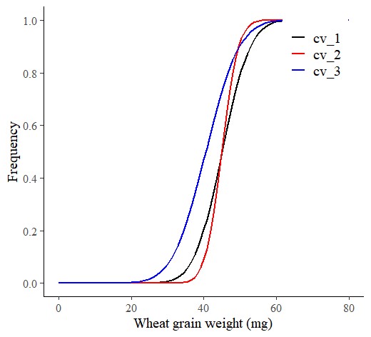
Next, I’ll use probdistz().
dataA= probdistz(df, env_cols= c("field","genotype"), yield_cols="grain_weight", smooth= TRUE)ggplot(data=subset(dataA, field=="up_state"), aes(x=grain_weight, y=smooth_cdf, color=genotype)) +
geom_line ()+
scale_color_manual(name= "Genotype", values = c("cv_1"="black", "cv_2"="red", "cv_3"="blue")) +
scale_x_continuous(breaks=seq(0,80,20), limits=c(0,80)) +
scale_y_continuous(breaks=seq(0,1,0.2), limits=c(0,1)) +
labs(x="Wheat grain weight (mg)", y="Frequency") +
theme_classic(base_size=15, base_family="serif") +
theme(legend.position=c(0.85, 0.85),
legend.title=element_blank(),
legend.key=element_rect(color="white", fill="white"),
legend.text=element_text(family="serif", face="plain", size=15, color= "Black"),
legend.background=element_rect(fill="white"),
axis.line=element_line(linewidth=0.5, colour="black"))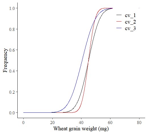
■ probdistz code for Z-distribution
probdistz() can provide z-distribution.
dataA= probdistz(df, env_cols= c("field","genotype"), yield_cols= c("grain_weight"), smooth= TRUE)ggplot(data=subset(dataA, field=="up_state"), aes(x=smooth_z, y=smooth_pdf, color=genotype)) +
geom_line ()+
scale_color_manual(name= "Genotype", values= c("cv_1"="black", "cv_2"="red", "cv_3"="blue")) +
scale_x_continuous(breaks=seq(-4,4,1), limits=c(-4,4)) +
scale_y_continuous(breaks=seq(0,0.2,0.05), limits=c(0,0.2)) +
labs(x="Z-score", y="Frequency") +
theme_classic(base_size=15, base_family="serif") +
theme(legend.position=c(0.85, 0.85),
legend.title=element_blank(),
legend.key=element_rect(color="white", fill="white"),
legend.text=element_text(family="serif", face="plain", size=15, color= "Black"),
legend.background=element_rect(fill="white"),
axis.line=element_line(linewidth=0.5, colour="black"))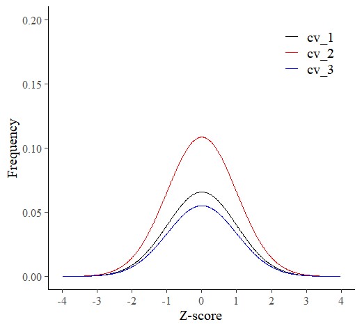
■ probdistz code (smooth= FALSE)
In probdistz() package, when selecting smooth= FALSE, it provides PDF, CDF and Z-score regarding the actual data, not predicting additional data based on 6σ.
dataA= probdistz(df, env_cols= c("field","genotype"), yield_cols="grain_weight", smooth= FALSE)ggplot(data=subset(dataA, field=="up_state"), aes(x=grain_weight, y=pdf_grain_weight, color=genotype)) +
geom_line ()+
scale_color_manual(name= "Genotype", values= c("cv_1"="black", "cv_2"="red", "cv_3"="blue")) +
scale_x_continuous(breaks=seq(0,80,20), limits=c(0,80)) +
scale_y_continuous(breaks=seq(0,0.15,0.03), limits=c(0,0.15)) +
labs(x="Wheat grain weight (mg)", y="Frequency") +
theme_classic(base_size=15, base_family="serif") +
theme(legend.position=c(0.85, 0.85),
legend.title=element_blank(),
legend.key=element_rect(color="white", fill="white"),
legend.text=element_text(family="serif", face="plain", size=15, color= "Black"),
legend.background=element_rect(fill="white"),
axis.line=element_line(linewidth=0.5, colour="black"))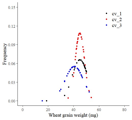
So, this graph is the same as the one created using Excel. If the data size increases, it will display a probability curve graph. This means that when using stat_function() and probdistz(), the estimation is based on the mean and standard deviation of the entire dataset. For probdistz(), I estimated it up to 6σ.
□ Github: https://github.com/agronomy4future/probdistz/blob/main/README.md
□ Code summary: https://github.com/agronomy4future/r_code/blob/main/Probability_Distribution_and_Z_Score_Calculation_Function_feat_probdistz.ipynb