Machine Learning: Predicting Values with Multiple Models- Part I
Machine learning (ML) is a field of artificial intelligence (AI) that enables computers to learn from and make predictions or decisions based on data. Rather than being explicitly programmed to perform a specific task, ML algorithms use data to identify patterns and make inferences or predictions.
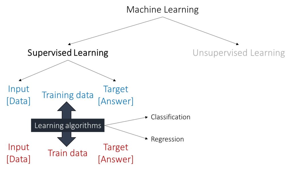
Machine Learning can be divided into supervised and unsupervised learning. In supervised learning, the model is trained on labeled data, which means the input data is paired with the correct output, and it can be further divided into classification and regression.
■ Machine Learning: How to Perform Classification with Different Models?
In classification, the model predicts categorical labels. Examples include spam detection (spam or not spam), image recognition (cat, dog, etc.), and medical diagnosis (disease present or not). In regression, the model predicts continuous values. Examples include predicting house prices, stock prices, or temperatures.
Let’s practice predicting values in machine learning using the following data. I use Python.
■ Data upload
import pandas as pd
import requests
from io import StringIO

github="https://raw.githubusercontent.com/agronomy4future/raw_data_practice/main/ML_Practice_Grain_Dimension.csv"
response=requests.get(github)
df=pd.read_csv(StringIO(response.text))

print(df.head(5))
  Genotype  Length_mm  Width_mm  Area_mm_2  GW_mg
0      cv1       4.86      2.12       7.56  14.44
1      cv1       5.01      1.94       7.25  13.67
2      cv1       5.54      1.97       7.99  15.55
3      cv1       3.84      1.99       5.86  10.32
4      cv1       5.30      2.06       8.04  15.66
First, I’ll convert categorical variables to numerical variables, such as 0, 1, etc. For example, I’ll change cv1 to 0 and cv5 to 4 in Genotype.
df['Genotype'] = df['Genotype'].replace({'cv1': 0, 'cv2': 1, 'cv3': 2, 'cv4': 3, 'cv5': 4})

print(df.head(5))
   Genotype  Length_mm  Width_mm  Area_mm_2  GW_mg
0         0       4.86      2.12       7.56  14.44
1         0       5.01      1.94       7.25  13.67
2         0       5.54      1.97       7.99  15.55
3         0       3.84      1.99       5.86  10.32
4         0       5.30      2.06       8.04  15.66
Next, I’ll distinguish from input and target data. Input data is actual data, and target data is answer
■ Data Splitting
In machine learning, data is typically divided into input data (features) and target data. Input data is the actual data used to make predictions. Each input feature represents a variable that can influence the target. Target data is the answer or outcome that you want to predict. Once trained, the model can be used to make predictions on new, unseen data.
In this case, I’ll choose data for ‘length’ and ‘width’ of grains to predict grain weights. Therefore, ‘length’ and ‘width’ will be input data, and grain weight will be target data.
# input
input= df.drop(columns=['Genotype','GW_mg','Area_mm_2'])

print(input.head(5))
   Length_mm  Width_mm
0       4.86      2.12
1       5.01      1.94
2       5.54      1.97
3       3.84      1.99
4       5.30      2.06

# target
target= df['GW_mg']

print(target.head(5))
0    14.44
1    13.67
2    15.55
3    10.32
4    15.66
Next, I’ll split the dataset into training and testing sets. By training the computer, it will learn to predict values. To achieve this, I will use train_test_split() to divide the data.
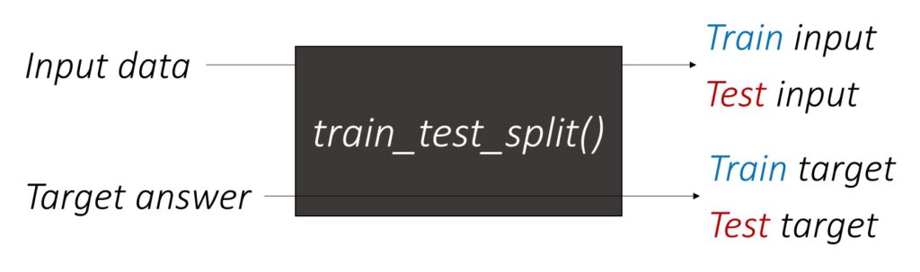
from sklearn.model_selection import train_test_split

train_input, test_input, train_target, test_target = train_test_split(input, target, test_size=0.3, random_state=42)
■ Machine Learning Algorithm
1. Random Forest
from sklearn.ensemble import RandomForestRegressor
rf= RandomForestRegressor()
rf_model= rf.fit(train_input, train_target)
accuracy= rf_model.score(test_input, test_target)

print("Accuracy:", accuracy)
Accuracy: 0.967082237064393
2. K-nearest neighbors
from sklearn.neighbors import KNeighborsRegressor
knr = KNeighborsRegressor()
knr_model = knr.fit(train_input, train_target)
accuracy = knr_model.score(test_input, test_target)

print("Accuracy:", accuracy)
Accuracy: 0.9632848876111081
3. Linear Regression
from sklearn.linear_model import LinearRegression
lr= LinearRegression ()
lr_model = lr.fit(train_input, train_target)
accuracy = lr_model.score(test_input, test_target)

print("Accuracy:", accuracy)
Accuracy: 0.877976186366542
4. Decision Tree
from sklearn.tree import DecisionTreeRegressor
dt = DecisionTreeRegressor()
dt_model= dt.fit(train_input, train_target)
accuracy = dt_model.score(test_input, test_target)

print("Accuracy:", accuracy)
Accuracy: 0.9544338125136431
5. Ridge regression
from sklearn.linear_model import Ridge
ridge = Ridge()
ridge_model= ridge.fit(train_input, train_target)
accuracy = ridge_model.score(test_input, test_target)

print("Accuracy:", accuracy)
Accuracy: 0.8779764868294875
6. Lasso regression
from sklearn.linear_model import Lasso
lasso = Lasso()
lasso_model= lasso.fit(train_input, train_target)
accuracy = lasso_model.score(test_input, test_target)

print("Accuracy:", accuracy)
Accuracy: 0.8479851709835504
Random forest shows the greatest accuracy, and therefore, I’ll choose it to predict grain weight.
| Model | Accuracy |
| Random Forest | 0.967 |
| K-nearest neighbors | 0.963 |
| Linear Regression | 0.878 |
| Decision Tree | 0.955 |
| Ridge | 0.878 |
| Lasso | 0.848 |
■ To verify the model
Now, I’ll use a new dataset to compare the actual grain weight with the grain weight predicted by the random forest model.
Let’s believe that after processing the machine learning model last year, I harvested crops this season and measured all the data for length, width, and grain area.
github="https://raw.githubusercontent.com/agronomy4future/raw_data_practice/main/ML_Practice_Grain_Dimension_Verifying.csv"
response=requests.get(github)
df1=pd.read_csv(StringIO(response.text))

print(df1.head(5))
  Genotype  Length_mm  Width_mm  Area_mm_2  GW_mg
0      cv3       6.40      3.40      15.50  37.46
1      cv3       7.46      3.68      19.81  51.82
2      cv3       7.14      3.75      19.50  50.76
3      cv3       6.60      3.40      15.90  38.75
4      cv3       7.02      3.70      18.92  48.77
df1['Genotype'] = df1['Genotype'].replace({'cv3': 2, 'cv4': 3, 'cv5': 4})
print(df1.head(5))
Genotype Length_mm Width_mm Area_mm_2 GW_mg
0 2 6.40 3.40 15.50 37.46
1 2 7.46 3.68 19.81 51.82
2 2 7.14 3.75 19.50 50.76
3 2 6.60 3.40 15.90 38.75
4 2 7.02 3.70 18.92 48.77Then, I’ll create input data for test dataset. This is because the training by random forest is done, and now we need to predict grain weight about the new dataset. So, the new dataset, df1, will be test data.
from sklearn.model_selection import train_test_split

train_input, test_input, train_target, test_target = train_test_split(input, target, test_size=0.3, random_state=42)
In above code to split train and test dataset, I provided the test data name as test_input and test_target. To distinguish from this, I’ll provide the test data name for a new dataset as test_input1 and test_target1.
# input
test_input1= df1.drop(columns=['Genotype','GW_mg','Area_mm_2'])

print(test_input1.head(5))
   Length_mm  Width_mm
0       6.40      3.40
1       7.46      3.68
2       7.14      3.75
3       6.60      3.40
4       7.02      3.70
# target
GW_mg = df1['GW_mg']
test_target1 = GW_mg
print(test_target1.head(5))
0 37.46
1 51.82
2 50.76
3 38.75
4 48.77Next, let’s do the same process for machine learning process to predict grain weight, but now the test dataset will be a new dataset this season.
Random Forest
from sklearn.ensemble import RandomForestRegressor
rf= RandomForestRegressor()
rf_model= rf.fit(train_input, train_target)
accuracy= rf_model.score(test_input1, test_target1)

print("Accuracy:", accuracy)
Accuracy: 0.8434369615301438
Using random forest model, when I predict grain weight for a new dataset, and the accuracy is 0.84. The accuracy is decreased when I use a new dataset in this season. When a machine learning model is trained on a specific dataset, it learns patterns and relationships within that training data. However, when a new, previously unseen dataset is introduced, the model’s performance often decreases.
■ To compare the actual and predicted grain weight
We have actual grain weight data for this season, so we can compare the actual and predicted grain weights.
print(test_input1.head(5))
   Length_mm  Width_mm
0       6.40      3.40
1       7.46      3.68
2       7.14      3.75
3       6.60      3.40
4       7.02      3.70
The test_input1 data consists of measurements I harvested this season, specifically choosing ‘length’ and ‘width’ to predict grain weight. I’ll use a Lasso model to predict grain weight using this ‘length’ and ‘width’ data.
y_pred= rf_model.predict(test_input1)

y_pred
42.13614,54.9686,55.22399333,44.01645802,51.78689821,50.2887288,43.88530894,58.325435,54.3813323,41.01634833,45.64443833,43.76950083,49.435095,48.9339544,34.50533361,54.39095,52.46250667,48.51996214,52.75912833,55.55805,55.48754333,56.23594381,58.4547,57.45136214,48.50953333,47.19934762,53.869175,54.72461,56.2707,57.61643333...
I’ll add this data to test_input1 with the new column name, ‘prediction.’
test_input1['prediction']= y_pred

print(test_input1.head(5))
   Length_mm  Width_mm  prediction
0       6.40      3.40   42.136140
1       7.46      3.68   54.968600
2       7.14      3.75   55.223993
3       6.60      3.40   44.016458
4       7.02      3.70   51.786898
and I’ll add actual grain weight data for this season.
test_input1['Grain_weight']= test_target1

print(test_input1.head(5))
   Length_mm  Width_mm  prediction  Grain_weight
0       6.40      3.40   42.136140         37.46
1       7.46      3.68   54.968600         51.82
2       7.14      3.75   55.223993         50.76
3       6.60      3.40   44.016458         38.75
4       7.02      3.70   51.786898         48.77
Great!! Now I have both actual and predicted grain weight data. I’ll export this data to my PC.
import pandas as pd
from google.colab import files

# Save the DataFrame to a CSV file
test_input1.to_csv('Grain_weight_2024.csv', index=False)

# Use the files module to download the file
files.download('Grain_weight_2024.csv')
I fitted the actual grain weight (column C) as x-axis and predicted grain weight (column D) as y-axis in Excel. The resulting figure is shown below.
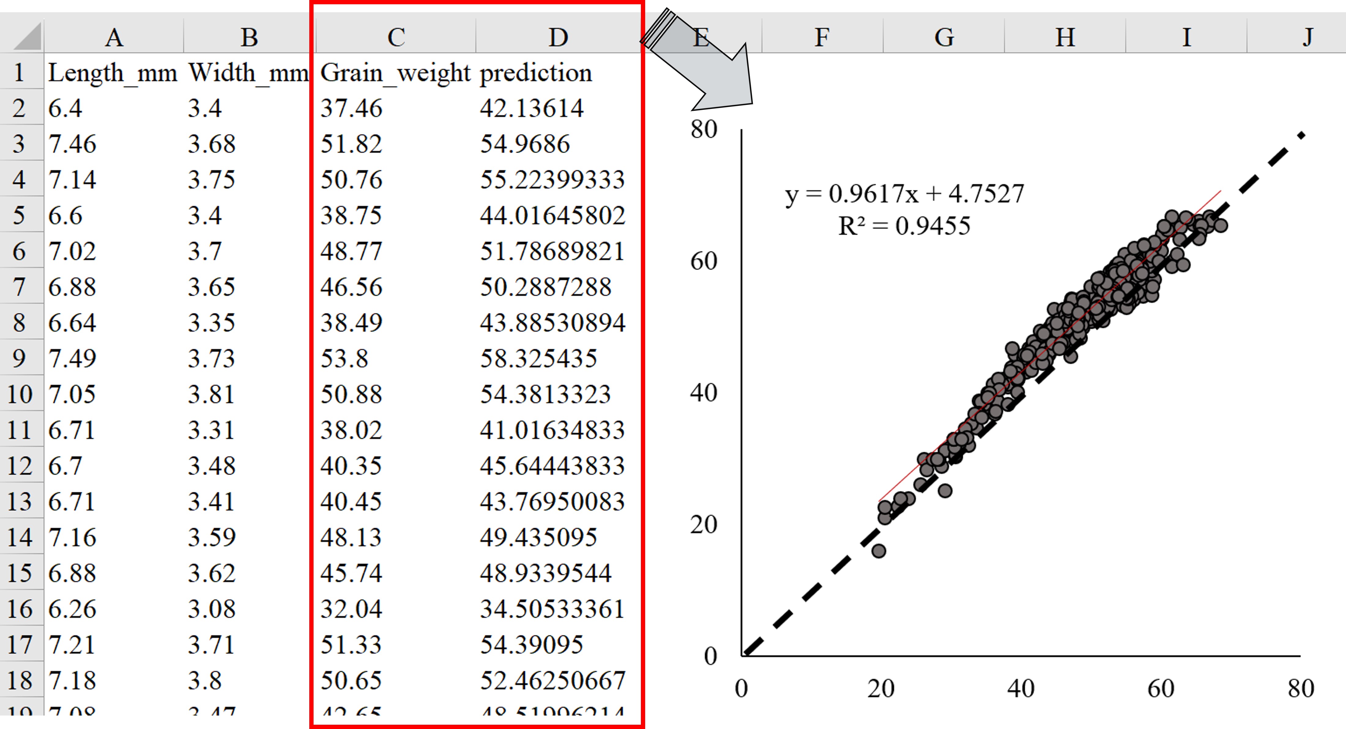
Let’s see this linear regression is statistically significant.
import statsmodels.api as sm
from statsmodels.formula.api import ols

regression= ols('prediction ~ Grain_weight', data=test_input1).fit()
regression_summary = regression.summary()
print(regression_summary)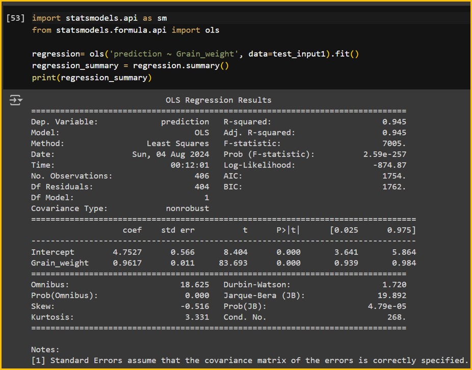
It’s significant. Let’s check R2
ANOVA=sm.stats.anova_lm(regression, typ=1)
print(f'ANOVA table: {ANOVA}')

r_squared = regression.rsquared
print(f'R-squared: {r_squared}')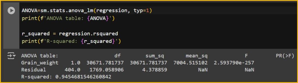
This prediction is quite accurate, showing a great R² value of 94.5%. Therefore, my machine learning process is quite successful.
Full code
# required package
import pandas as pd
import requests
from io import StringIO
from sklearn.model_selection import train_test_split
from sklearn.ensemble import RandomForestRegressor
import statsmodels.api as sm
from statsmodels.formula.api import ols

# data upload
github="https://raw.githubusercontent.com/agronomy4future/raw_data_practice/main/ML_Practice_Grain_Dimension.csv"
response=requests.get(github)
df=pd.read_csv(StringIO(response.text))
df['Genotype'] = df['Genotype'].replace({'cv1': 0, 'cv2': 1, 'cv3': 2, 'cv4': 3, 'cv5': 4})

# data splitting
input= df.drop(columns=['Genotype','GW_mg','Area_mm_2'])
target= df['GW_mg']
train_input, test_input, train_target, test_target = train_test_split(input, target, test_size=0.3, random_state=42)

# modeling
rf= RandomForestRegressor()
rf_model= rf.fit(train_input, train_target)
accuracy= rf_model.score(test_input, test_target)

# data upload (new dataset)
github="https://raw.githubusercontent.com/agronomy4future/raw_data_practice/main/ML_Practice_Grain_Dimension_Verifying.csv"
response=requests.get(github)
df1=pd.read_csv(StringIO(response.text))
df1['Genotype'] = df1['Genotype'].replace({'cv3': 2, 'cv4': 3, 'cv5': 4})

# data splitting
test_input1= df1.drop(columns=['Genotype','GW_mg','Area_mm_2'])
GW_mg = df1['GW_mg']
test_target1 = GW_mg

# modeling
from sklearn.ensemble import RandomForestRegressor
rf= RandomForestRegressor()
rf_model= rf.fit(train_input, train_target)
accuracy= rf_model.score(test_input1, test_target1)

# prediction
y_pred= rf_model.predict(test_input1)
test_input1['prediction']= y_pred
test_input1['Grain_weight']= test_target1

# statistics
regression= ols('prediction ~ Grain_weight', data=test_input1).fit()
regression_summary = regression.summary()
print(regression_summary)

ANOVA=sm.stats.anova_lm(regression, typ=1)
print(f'ANOVA table: {ANOVA}')

r_squared = regression.rsquared
print(f'R-squared: {r_squared}')