Machine Learning: How to Perform Classification with Different Models?
Machine learning (ML) is a field of artificial intelligence (AI) that enables computers to learn from and make predictions or decisions based on data. Rather than being explicitly programmed to perform a specific task, ML algorithms use data to identify patterns and make inferences or predictions.
What is Classification in Machine Learning?
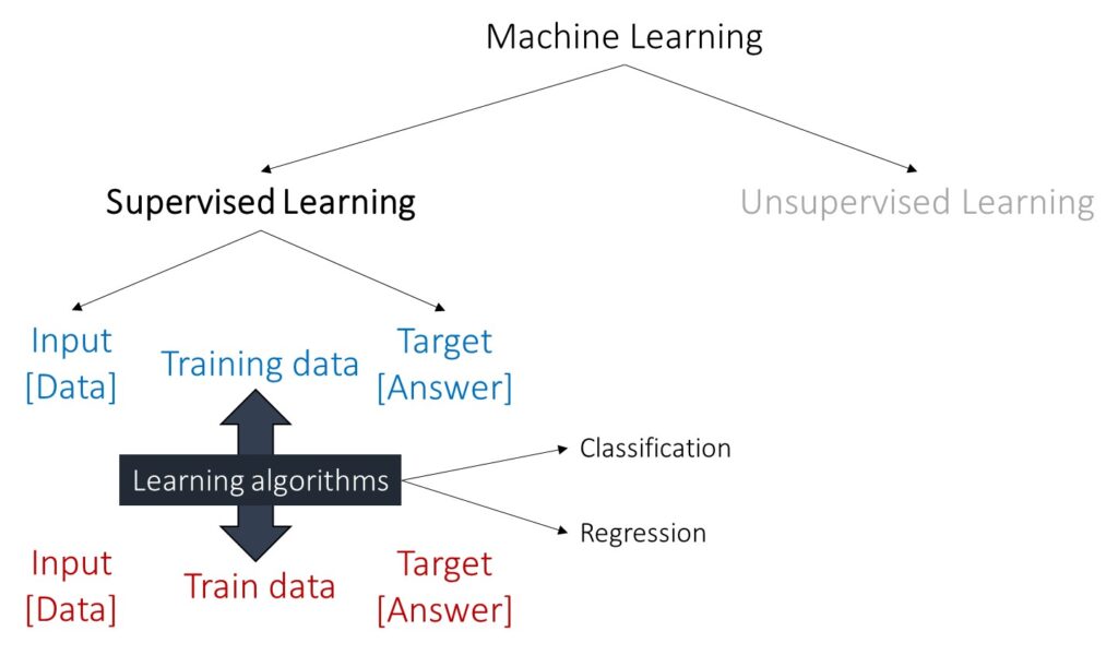
Classification is a type of supervised learning where the goal is to categorize data into predefined classes. For example, classifying emails as “spam” or “not spam.” Different models can be used for classification
■ Logistic Regression: A simple model for binary classification problems.
■ Decision Trees: Models that split data into branches to make predictions.
■ Random Forest: An ensemble of decision trees that improves accuracy and robustness.
■ Support Vector Machines (SVM): Models that find the best boundary between classes.
■ K-Nearest Neighbors (KNN): Classifies based on the majority class among the nearest neighbors.
■ Neural Networks: Complex models capable of learning from large datasets and capturing intricate patterns.
Let’s practice classification in machine learning using the following data. I use Python.
import pandas as pd
import requests
from io import StringIO

github="https://raw.githubusercontent.com/agronomy4future/raw_data_practice/main/carbon_nitrogen_emission.csv"
response=requests.get(github)
df=pd.read_csv(StringIO(response.text))

print(df [:5])
   Season     Crop  Day  Carbon_flux  Nitrogen_flux
0    2015  Soybean    0    13.659544       0.012144
1    2015  Soybean    1    28.511196       0.024585
2    2015  Soybean    2    44.554958       0.037320
3    2015  Soybean    3    61.790819       0.050352
4    2015  Soybean    4    80.218788       0.063689
.
.
.
This data measures cumulative carbon and nitrogen flux over time in different seasons. Each season had different crops: sorghum or soybean. I am interested in determining which crop was grown based on the cumulative carbon and nitrogen flux. Therefore, I would like to use a machine learning model.
import matplotlib.pyplot as plt

# Create a mask for each crop type
sorghum_mask = df['Crop'] == 'Sorghum'
soybean_mask = df['Crop'] == 'Soybean'

# Plot the scatter plot for Sorghum in red
plt.scatter(df[sorghum_mask]['Carbon_flux'], df[sorghum_mask]['Nitrogen_flux'], color='red', label='Sorghum')

# Plot the scatter plot for Soybean in blue
plt.scatter(df[soybean_mask]['Carbon_flux'], df[soybean_mask]['Nitrogen_flux'], color='blue', label='Soybean')

# Add labels and legend
plt.xlabel('Carbon')
plt.ylabel('Nitrogen')
plt.legend()
plt.show()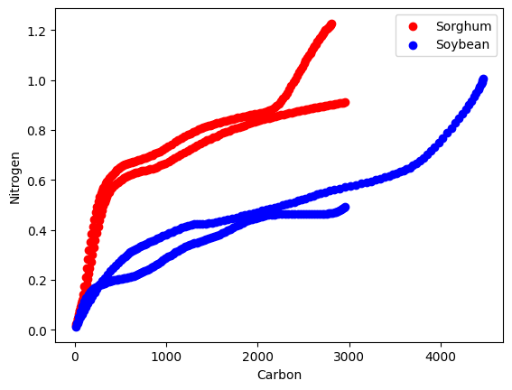
First, I’ll identify the variables that might affect the differences between sorghum and soybean. As shown in the graph above, carbon and nitrogen fluxes are distinct between sorghum and soybean, so I’ll include these variables. Additionally, I believe that cumulative days are important, so I’ll include this variable as well.
import numpy as np

Carbon_flux = df['Carbon_flux']
Nitrogen_flux = df['Nitrogen_flux']
Day= df['Day']
GHGs_data = np.column_stack((Carbon_flux, Nitrogen_flux, Day))

print(GHGs_data[:5])
print(GHGs_data.shape)

[[1.36595437e+01 1.21444200e-02 0.00000000e+00]
 [2.85111963e+01 2.45845800e-02 1.00000000e+00]
 [4.45549577e+01 3.73204800e-02 2.00000000e+00]
 [6.17908185e+01 5.03521200e-02 3.00000000e+00]
 [8.02187881e+01 6.36890400e-02 4.00000000e+00]]
(519, 3)
The input data consists of 519 rows and 3 columns. Typically, rows are referred to as samples, and columns are referred to as features (e.g., carbon flux, nitrogen flux, and measuring day).
We also need to create a target answer, which provides the computer with both the input data and the corresponding answer. In this case, since we want to classify sorghum and soybean using different variables, the target variable will be the actual crop type for each sample. Since the computer does not understand the text labels “sorghum” and “soybean” directly, we need to convert these labels into binary values, such as 0 and 1.
crop_column = df['Crop']
target = crop_column.replace({'Sorghum': 0, 'Soybean': 1})

print(target[:5])
0    1
1    1
2    1
3    1
4    1
■ Dividing train and test data set
Now, we need to divide these samples into training and testing datasets. We can use the train_test_split() function for this purpose.
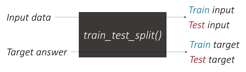
from sklearn.model_selection import train_test_split

train_GHGs, test_GHGs, train_target, test_target = train_test_split(GHGs_data, target, test_size=0.2, random_state=42)
I divided the data into 80% for training and 20% for testing.
print(train_GHGs.shape, test_GHGs.shape)
print(train_target.shape, test_target.shape)

(415, 3) (104, 3)
(415,) (104,)
Consequently, the training dataset consists of 415 samples, while the testing dataset contains 104 samples.
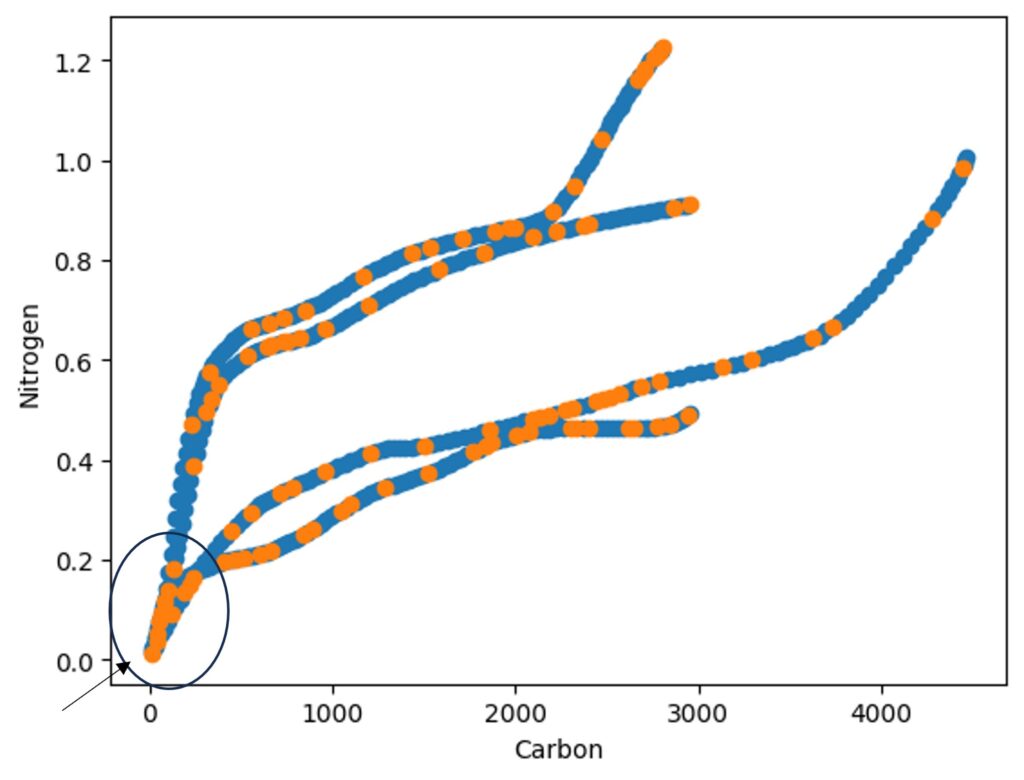
import matplotlib.pyplot as plt
plt.scatter (train_GHGs[:,0], train_GHGs[:,1])
plt.scatter (test_GHGs[:,0], test_GHGs[:,1])
plt.xlabel('Carbon')
plt.ylabel('Nitrogen')
plt.show()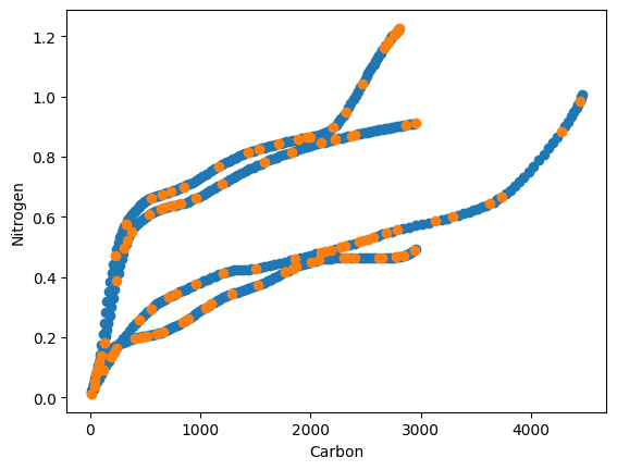
The blue color represents the training data, and the orange color represents the testing data. The data has been randomly divided.
■ Machine Learning Algorithm
1. K-Nearest Neighbors (KNN)
from sklearn.neighbors import KNeighborsClassifier
KNN = KNeighborsClassifier()
KNN_model = KNN.fit(train_GHGs, train_target)
accuracy = KNN_model.score(test_GHGs, test_target)
print("Accuracy:", accuracy)

Accuracy: 0.5384615384615384
2. Linear Regression
from sklearn.linear_model import LinearRegression
LinearRegression= LinearRegression ()
LinearRegression_model = LinearRegression.fit(train_GHGs, train_target)
accuracy = LinearRegression_model.score(test_GHGs, test_target)
print("Accuracy:", accuracy)

Accuracy: 0.7640997636566816
3. Random Forest
from sklearn.ensemble import RandomForestClassifier
RandomForest = RandomForestClassifier()
RandomForest_model= RandomForest.fit(train_GHGs, train_target)
accuracy = RandomForest_model.score(test_GHGs, test_target)
print("Accuracy:", accuracy)

Accuracy: 0.9615384615384616
4. Logistic Regression
from sklearn.linear_model import LogisticRegression
LogisticRegression = LogisticRegression()
LogisticRegression_model= LogisticRegression.fit(train_GHGs, train_target)
accuracy = LogisticRegression_model.score(test_GHGs, test_target)
print("Accuracy:", accuracy)

Accuracy: 0.9134615384615384
5. Decision Tree
from sklearn.tree import DecisionTreeClassifier
DecisionTree = DecisionTreeClassifier()
DecisionTree_model= DecisionTree.fit(train_GHGs, train_target)
accuracy = DecisionTree_model.score(test_GHGs, test_target)
print("Accuracy:", accuracy)

Accuracy: 0.9326923076923077
6. Support Vector Machines (SVM)
from sklearn.svm import SVC
SVC = SVC()
SVC_model= SVC.fit(train_GHGs, train_target)
accuracy = SVC_model.score(test_GHGs, test_target)
print("Accuracy:", accuracy)

Accuracy: 0.5192307692307693
7. Gaussian
from sklearn.naive_bayes import GaussianNB
Gaussian = GaussianNB()
Gaussian_model= Gaussian.fit(train_GHGs, train_target)
accuracy = Gaussian_model.score(test_GHGs, test_target)
print("Accuracy:", accuracy)

Accuracy: 0.9134615384615384
When using Random Forest, it shows the greatest accuracy.
■ Modfying data group [adding new variables]
At the early measuring stage, the GHG emissions from sorghum and soybean were quite similar, which I believe may have reduced the accuracy. Therefore, I want to add a new variable for carbon flux groups using the following code.
df['C_Group'] = df['Carbon_flux'].apply(
    lambda x: '0' if x < 100 else
              '1' if 100 <= x < 1000 else
              '2' if 1000 <= x < 2000 else
              '3' if 2000 <= x < 3000 else
              '4' if 3000 <= x < 4000 else
              '5'
)
and I’ll add this new variable to the input data.
Carbon_flux = df['Carbon_flux']
Nitrogen_flux = df['Nitrogen_flux']
Day= df['Day']
C_group= df['C_Group']
GHGs_data = np.column_stack((Carbon_flux, Nitrogen_flux, Day, C_group))
and will run the same code.
[K-nearest neighbors] Accuracy: 0.5384615384615384
[Linear Regression] Accuracy: 0.7658031541434641
[Random Forest] Accuracy: 0.9711538461538461
[Logistic Regression] Accuracy: 0.9519230769230769
[Decision Tree] Accuracy: 0.9519230769230769
[GaussianNB] Accuracy: 0.9230769230769231
[Support Vector Machines] Accuracy: 0.5192307692307693
[Gaussian] Accuracy: 0.9423076923076923
The accuracy is slightly changed. Actually, when you add a new variable (or feature) to your dataset in a machine learning process, several things can happen, which might affect the model’s accuracy:
- Better Pattern Recognition: If the new variable provides useful information that helps the model make better predictions, you might see an improvement in accuracy. Essentially, the model can learn a more accurate pattern or relationship between features and the target variable.
- Overfitting Risk: Adding more features can also increase the risk of overfitting. Overfitting occurs when a model learns the noise in the training data rather than the underlying pattern, leading to poor generalization on new, unseen data. This is more likely if the new variable doesn’t add much new information or if the dataset is small.
- Dimensionality and Complexity: Introducing additional features increases the dimensionality of the data, which can sometimes make it harder for the model to learn effectively. This is known as the “curse of dimensionality.” With more features, the model might require more sophisticated techniques or more data to perform well.
- Feature Importance: The impact of a new variable on accuracy can also depend on its relevance and importance in the context of other features. If the new variable has a strong relationship with the target variable, it can significantly improve the model’s performance.
In summary, adding a new variable can help the model find better patterns if the feature is relevant and informative. However, it’s essential to carefully evaluate the model to ensure that the improvement in accuracy is genuine and not due to overfitting or other issues related to the complexity of the model. Techniques like cross-validation can help assess whether the addition of new features genuinely improves the model’s performance on unseen data.