What is the statistical method for comparing whether the slopes and y-intercepts in a regression model are the same or not (Feat. ANCOVA using R and SAS)?
To gain a basic understanding of the topic, I recommend reading the following posts.
Analysis of Covariance (ANCOVA)
- What is ANCOVA (1/3)? The basic concept
- What is ANCOVA (2/3)? How to interpret Parameter Estimates
- What is ANCOVA (3/3)? The common slope and adjusted mean
I have a dataset as shown below, and I would like to analyze crop yield, and height based on different fertilizer types (Control, Slow-release, and Fast-release). The experimental design is a Completely Randomized Design (CRD) with 10 replicates.
| Rep | Fertilizer | Yield | Height | Fertilizer | Yield | Height | Fertilizer | Yield | Height |
| 1 | Control | 12.2 | 45.0 | Slow | 16.6 | 63.0 | Fast | 9.5 | 52.0 |
| 2 | Control | 12.4 | 52.0 | Slow | 15.8 | 50.0 | Fast | 9.5 | 54.0 |
| 3 | Control | 11.9 | 42.0 | Slow | 16.5 | 63.0 | Fast | 9.6 | 58.0 |
| 4 | Control | 11.3 | 35.0 | Slow | 15.0 | 33.0 | Fast | 8.8 | 45.0 |
| 5 | Control | 11.8 | 40.0 | Slow | 15.4 | 38.0 | Fast | 9.5 | 57.0 |
| 6 | Control | 12.1 | 48.0 | Slow | 15.6 | 45.0 | Fast | 9.8 | 62.0 |
| 7 | Control | 13.1 | 60.0 | Slow | 15.8 | 50.0 | Fast | 9.1 | 52.0 |
| 8 | Control | 12.7 | 61.0 | Slow | 15.8 | 48.0 | Fast | 10.3 | 67.0 |
| 9 | Control | 12.4 | 50.0 | Slow | 16.0 | 50.0 | Fast | 9.5 | 55.0 |
| 10 | Control | 11.4 | 33.0 | Slow | 15.8 | 49.0 | Fast | 8.5 | 40.0 |
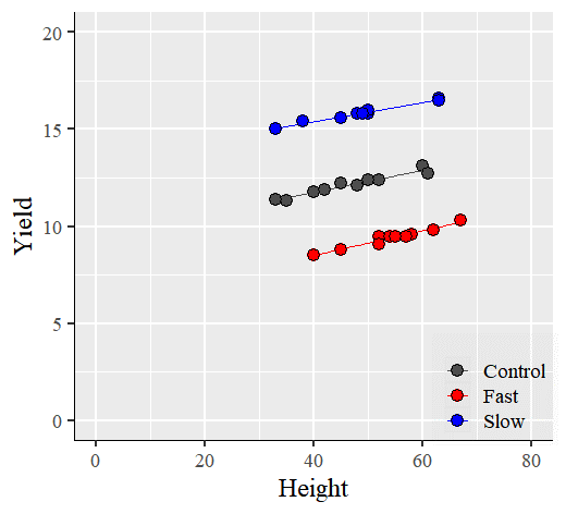
Now, I’ll draw a linear regression line between height and yield for each fertilizer treatment. I use R.
# to upload data
library (readr)
github="https://raw.githubusercontent.com/agronomy4future/raw_data_practice/main/Fertilizer%20(One%20Way%20ANOVA).csv"
dataA=data.frame(read_csv(url(github),show_col_types=FALSE))

# to draw a graph
library (ggplot2)
ggplot(data=dataA, aes(x=Height, y=Yield))+
  stat_smooth(aes(group=Fertilizer, color=Fertilizer), method='lm',
              linetype=1, se=FALSE, formula=y~x, linewidth=0.5) +
  geom_point(aes(fill=Fertilizer,shape=Fertilizer), size=4)+
  scale_fill_manual(values=c("grey30","red","blue"))+
  scale_color_manual(values=c("grey30","red","blue"))+
  scale_shape_manual(values=c(21,21,21))+
  scale_x_continuous(breaks=seq(0,80,20),limits=c(0,80))+
  scale_y_continuous(breaks=seq(0,20,5),limits=c(0,20))+
  labs(x="Height", x="Yield") +
  theme_grey(base_size=18, base_family="serif")+
  theme(legend.position=c(0.88,0.12),
        legend.title=element_blank(),
        legend.key=element_rect(color=alpha("grey",.05),
                   fill=alpha("grey",.05)),
        legend.background=element_rect(fill=alpha("grey",.05)),
        axis.line=element_line(linewidth=0.5, colour="black"))+
  windows(width=5.5, height=5)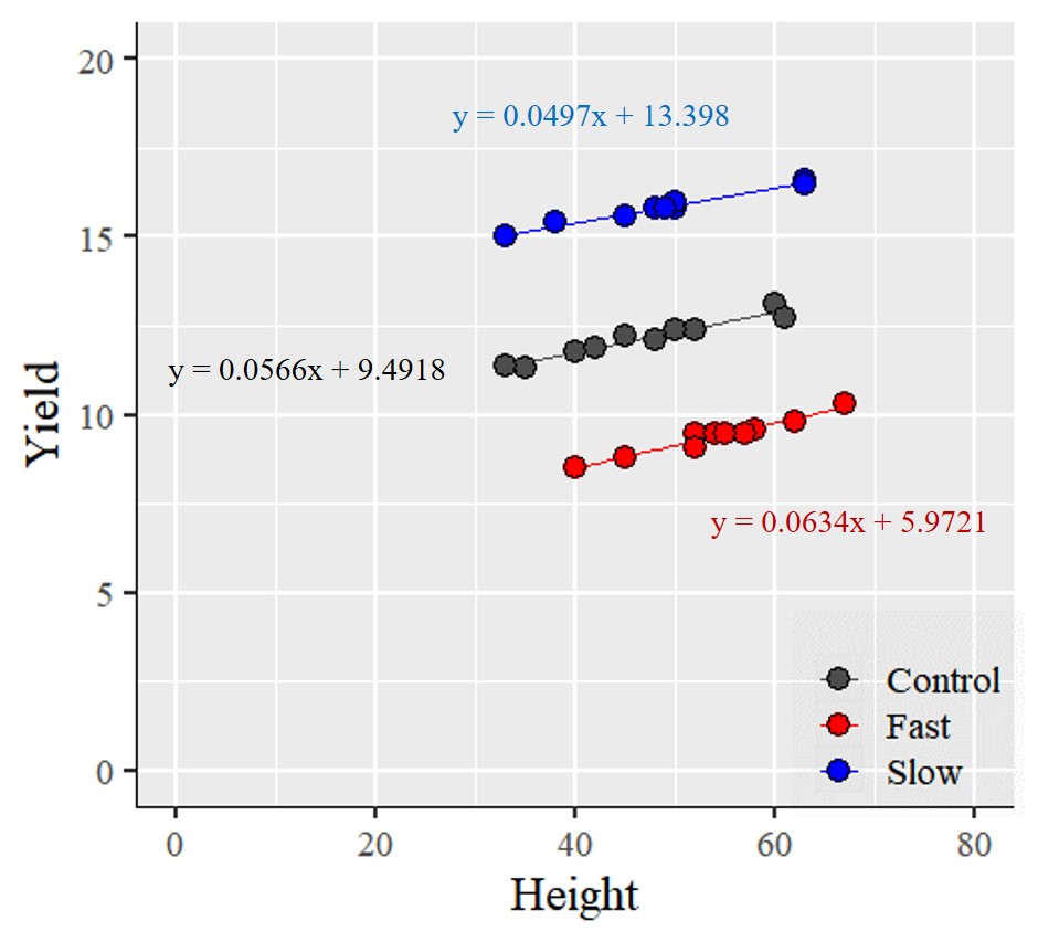
Now, I am interested in whether these three lines are parallel or not, in other words, whether their slopes are the same or not. The linear model equation for each fertilizer treatment is shown below.
Control: y = 0.0566x + 9.4918
Fast: y = 0.0634x + 5.9721
Slow: y = 0.0497x + 13.398
First, I’ll check the each slope is significant.
summary(lm(Yield~Height, data=subset(dataA, Fertilizer=="Control")))
summary(lm(Yield~Height, data=subset(dataA, Fertilizer=="Fast")))
summary(lm(Yield~Height, data=subset(dataA, Fertilizer=="Slow")))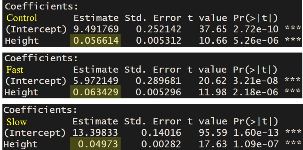
All slopes are significant (i.e., they are not equal to zero). Now, I would like to determine whether the slopes of these three lines are the same or not. To compare the slopes, I will conduct an Analysis of Covariance (ANCOVA).
Null hypothesis for ANCOVA
ANCOVA (Analysis of Covariance) is a statistical method to compare the means of two or more groups, controlling for the effects of one or more continuous variables (known as covariates) that may influence the dependent variable. ANCOVA combines the features of both analysis of variance (ANOVA) and regression analysis.
The reason for using ANCOVA to compare whether slopes are parallel or not is that the null hypothesis of ANCOVA is typically that there are no significant differences in the means of the groups after controlling for the effects of the covariate(s). This means that the covariate(s) is held constant, and any differences between the groups are assumed to be due to the independent variable(s) being compared.
In the relationship between the covariate and the dependent variable (y), if the slopes are parallel among treatments, it means that the effect of the covariate on the dependent variable is consistent across the groups being compared. However, it is important to note that the parallel slopes do not necessarily imply that the covariate has no effect on the dependent variable. Instead, the covariate may still have a significant impact on the dependent variable overall, but it is controlled for in the analysis so that any differences between the groups are not confounded by the covariate.
Once the first null hypothesis of ANCOVA is accepted, the second null hypothesis is that the intercepts of the regression lines (or ‘the adjusted means‘ among treatments) are all the same. This means that there are no significant differences in the dependent variable between treatments being compared, after adjusting for the effects of the covariate(s). The acceptance of the second null hypothesis suggests that any observed differences between treatments are solely due to the independent variable(s) being compared, and not influenced by the covariate(s).
For more details, please see the below post.
What is ANCOVA (3/3)? The common slope and adjusted mean
If you have followed the post above carefully, you would be able to calculate the adjusted mean
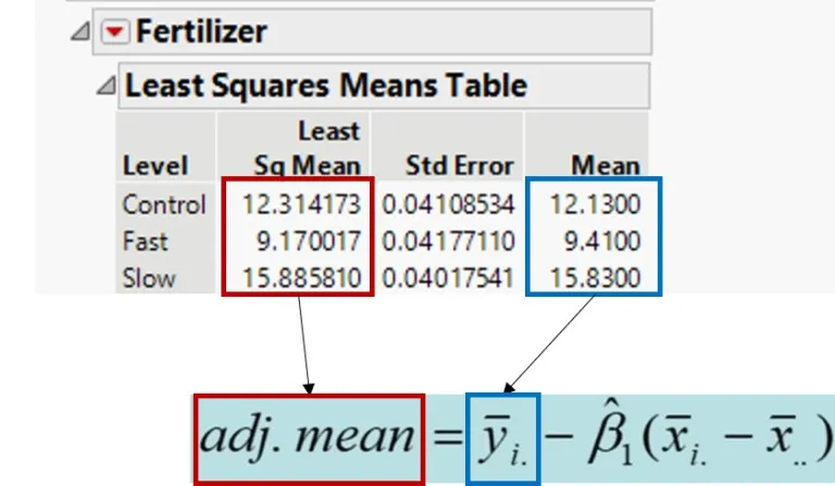
^β indicates the common slope and (x̄i. – x̄..) indicates the effect of the covariate. In the above post, I introduce how to obtain ^β, and (x̄i. – x̄..).
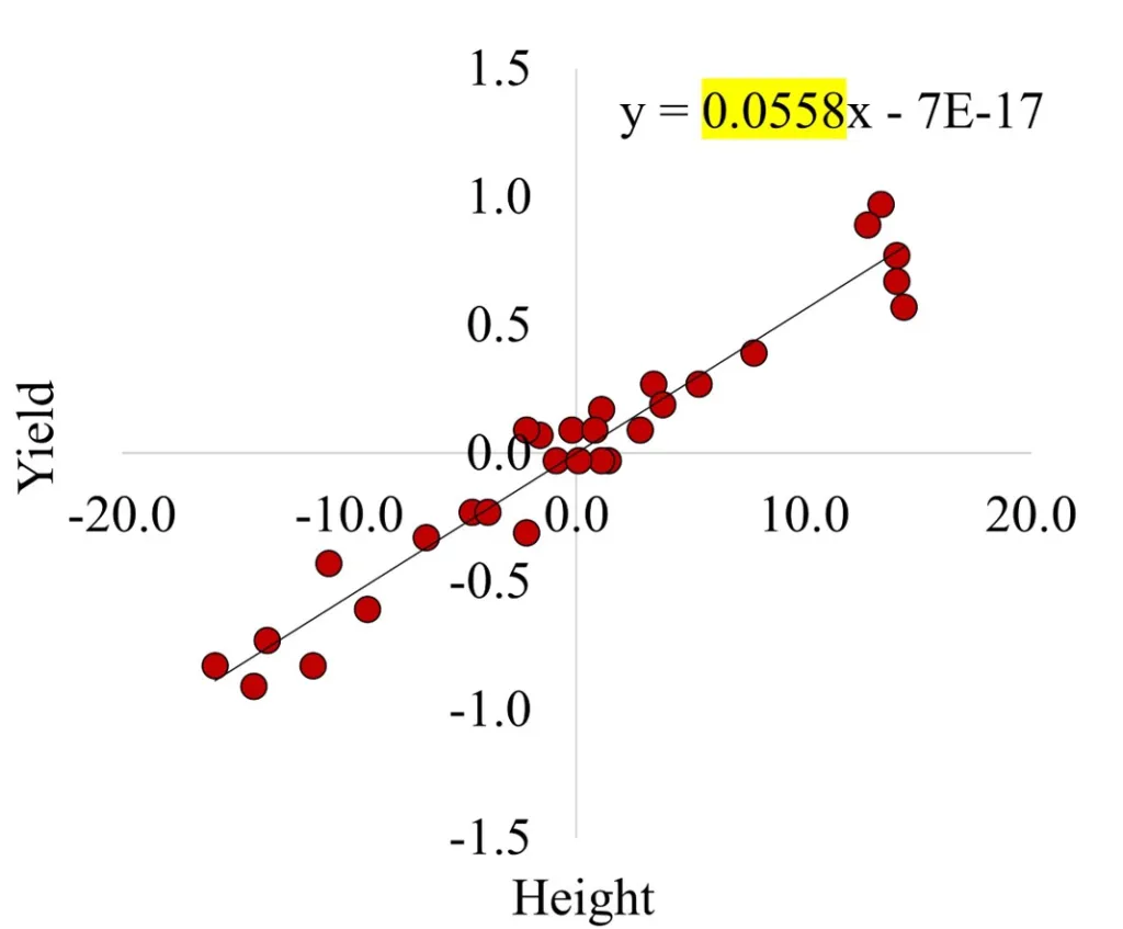
I calculated ^β as 0.0558 and the effect of covariate (x̄i. – x̄..) was calculated as
Control: -3.3
Fast: 4.3
Slow: -1.0
Therefore, the adjusted mean of yield will be
Control= 12.13 – 0.0558 * (-3.3) = 12.31
Fast= 9.41 – 0.0558 * (4.3) = 9.17
Slow= 15.83 – 0.0558 * (-1.0) = 15.89
With that basic background knowledge, let’s statistically test whether the slopes are the same or not.
Analysis of Covariance using R
First, I will demonstrate how to perform ANCOVA using R. To start, let’s upload the data. You can use the code below to copy and paste the data into your R script to upload data.
library (readr)
github="https://raw.githubusercontent.com/agronomy4future/raw_data_practice/main/Fertilizer%20(One%20Way%20ANOVA).csv"
dataA=data.frame(read_csv(url(github),show_col_types=FALSE))
1) Slopes
To determine whether the slopes are the same or different, I will test for interactions between height and fertilizer.
#install.packages("car")
library(car)
ancova_model= lm (Yield ~ Height + Fertilizer + Height:Fertilizer,
                  data=dataA)
Anova(ancova_model, type="II")
Since the interaction is not significant, the slopes among the fertilizers are not significantly different. This indicates that the model assumes the slopes of the regression lines are equal. At first glance, the slopes in the graph below may look similar, but our statistical analysis has shown that they are in fact parallel.

2) Y intercepts
Next, I am interested in testing whether the y-intercepts are the same or different.
ancova_model2= lm (Yield ~ Height + Fertilizer, data=dataA)
Anova(ancova_model2, type="II")
Since the interaction term is not included in this model, it assumes that the slopes of the regression lines are equal.

The independent variable (Fertilizer) is significant, so the intercepts among fertilizers are different.
3) Parameter estimates
Now, I’d like to see the common slope and the adjusted means. So I add below code.
ancova_model2= lm (Yield ~ Height + Fertilizer, data=dataA)
Anova(ancova_model2, type="II")
summary(ancova_model2)
The common slope is 0.0558 which is the same as I caclulated by hand, and the mean of height (covariate) is 49.9 (see the post; What is ANCOVA (3/3)? The common slope and adjusted mean).

Now, let’s estimate yield (a.k.a the adjusted mean).
Control: 9.529 + 0.0558 * 49.9 ≈ 12.31
Fast: 9.529 -3.144 + 0.0558* 49.9 ≈ 9.17
Slow: 9.529 + 3.572 + 0.0558 * 49.9 ≈ 15.89
This concept is a Generalized Linear Model (GLM). It’s the same value that I presented using JMP in the post titled; What is ANCOVA (3/3)? The common slope and adjusted mean).

Under parameter estimates, 0.0558 represents the common slope, and 9.529 represents the y-intercept for the regression line of the Fertilizer [Control]. The y-intercept for the regression line of the Fertilizer [Slow] is 3.571, which means the y intercept for Fertilizer [Slow] is 3.571 higher than Fertilizer [Control]. In the same way, the y intercept for Fertilizer [Fast] is -3.144 less than Fertilizer [Control].
Therefore, the conslusion is like below.
The effect of crop height (covariate) on yield (dependent variable) is consistent across the fertilizers being compared. However, the covariate has a significant impact on yield (the common slope, 0.0558 is significant), but any differences among fertilizers are not confounded by the covariate because there are significant differences in fertilizers.
If you have a full understanding of these concepts, you can simply use the code below.
library(car)
ancova_model=aov(Yield ~ Fertilizer + Height, data=dataA)
Anova(ancova_model, type="III")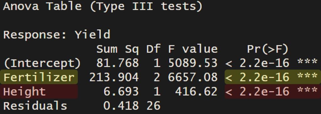
In this ANCOVA model, height (covariate) is highly significant (p<.001), indicating that crop yield is affected by crop height. However, even when height is included as a covariate, fertilizer remains highly significant (p<.001). This suggests that there are differences in crop yield among fertilizer types beyond those attributable to crop height.
Analysis of Covariance using SAS
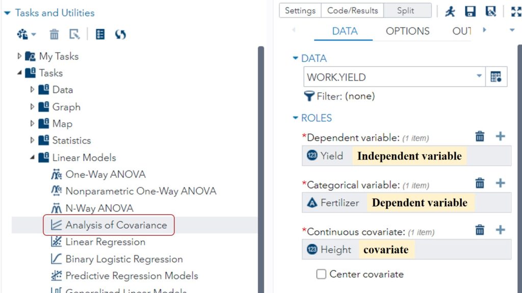
I will also introduce the same process that I showed using R, but this time with SAS. In SAS Studio, select the method as ‘Analysis of Covariance’ and input the independent, dependent, and covariate variables into the correct positions.
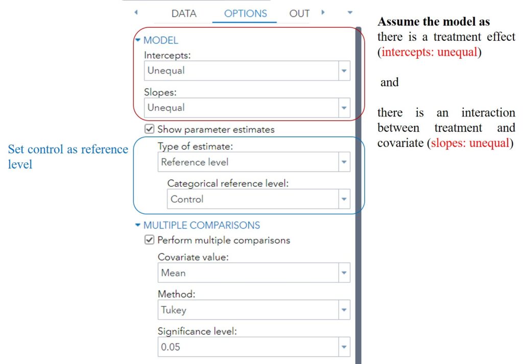
In the Options tab, specify the model. Choose ‘Unequal intercepts’ (assuming that the fertilizer treatment is significant) and ‘Unequal slopes’ (assuming that there is an interaction between the fertilizer and covariate).
Below is the outcome, which is the same result as the one provided by R.
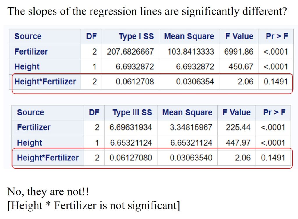
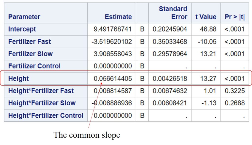
Below is the SAS code for the model described above.
proc glm data=WORK.YIELD;
	class Fertilizer  (ref='Control');
	model Yield=Fertilizer Height Height * Fertilizer / solution;
	lsmeans Fertilizer / adjust=tukey pdiff alpha=.05;
quit;
Based on our analysis, we have determined that there is no interaction (the slopes are parallel). Therefore, the following model assumes that the regression lines have equal slopes. To implement this model in SAS Studio, simply change ‘Unequal slopes’ to ‘Equal slopes’.
proc glm data=WORK.YIELD;
	class Fertilizer  (ref='Control');
	model Yield=Fertilizer Height / solution;
	lsmeans Fertilizer / adjust=tukey pdiff alpha=.05;
quit;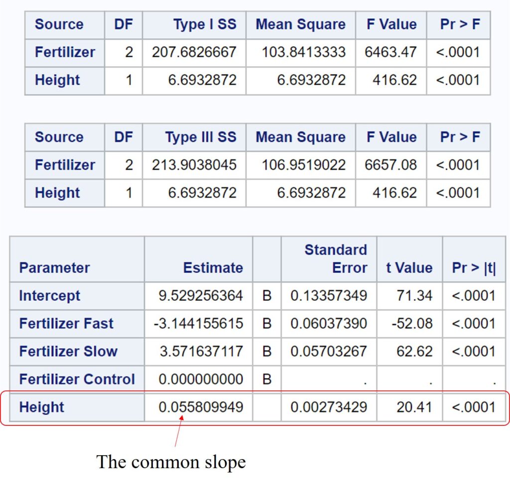
Now, the common slope and the adjusted mean is the as R provided.
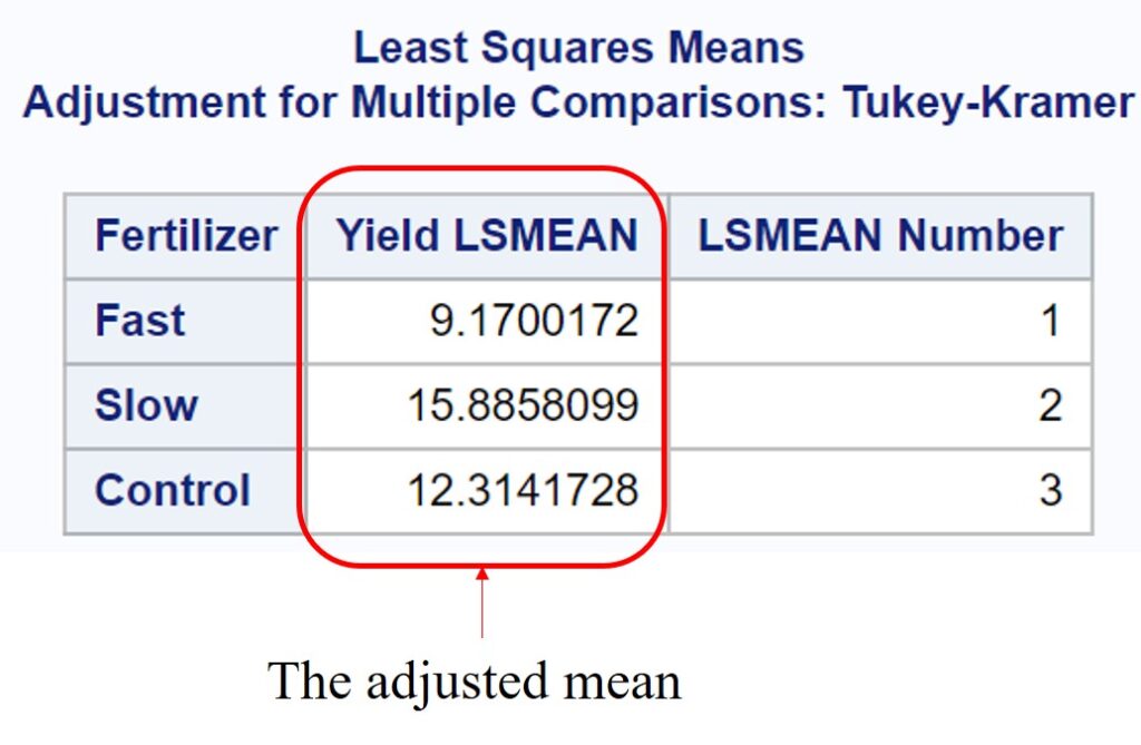
Are the intercepts of the regression lines (or ‘the adjusted means‘ among treatments) all the same?
No, it isn’t!! Fertilizer is significant (p<.0001), and the adjusted mean is also different.